In a sequence of articles we compare different NLP techniques to show you how we get valuable information from unstructured text. About a year ago we gathered reviews on Dutch restaurants. We were wondering whether ‘the wisdom of the crowd’ — reviews from restaurant visitors — could be used to predict which restaurants are most likely to receive a new Michelin-star. Read this post to see how that worked out. We used topic modeling as our primary tool to extract information from the review texts and combined that with predictive modeling techniques to end up with our predictions.
We got a lot of attention with our predictions and also questions about how we did the text analysis part. To answer these questions, we explain our approach in more detail in a series of articles on NLP. But we didn’t stop exploring NLP techniques after our publication, and we also like to share insights from adding more novel NLP techniques. More specifically we will use two types of word embeddings — a classic Word2Vec model and a GLoVe embedding model — we’ll use transfer learning with pretrained word embeddings and we use BERT. We compare the added value of these advanced NLP techniques to our baseline topic model on the same dataset. By showing what we did and how we did it, we hope to guide others that are keen to use textual data for their own data science endeavours.
In a previous article from our NLP series we have introduced you to Word Embeddings using a classic Word2Vec model and a GloVe model. These embeddings are useful in capturing semantic similarities on the words in your documents, in our case restaurant reviews. At face value the Word2Vec model seemed less promissing than the GloVe model. In this article we will use the embedding matrixes for both techniques for predicting which restaurant is most likely to receive a new Michelin star. This will shed a more quantitative light on which embedding model is better for downstream NLP prediction tasks. But we won’t stop there, we will also introduce Transfer Learning: using knowledge gained elsewhere (and embedding model trained on the Wikipedia Corpus) and apply it here. And we compare the prediction results using word embeddings with the Michelin predictions using topic modeling.
In this article we use Word Embedding for predicting which restaurant is more likely to receive a next Michelin star. Our prediction models will use our own trained word embeddings and we will also use a large pre-trained Wikipedia embedding.
Setting up our context
We enable our workbook with the required packages and data to perform our word embedding. AzureStor and R.utils are needed for saving model results from our Azure blob storage account and the R.utils package is used for unpacking pre-trained word embedding models. Tidyverse is the data wrangling and visualization toolkit created by the R legend Hadley Wickham. Tidytext is a ‘tidy’ R package focused on using text. Keras has become the centerpiece of our blog series. It is a popular package for building neural networks, a user friendly interface connected to the Tensorflow back-end.
Load preprocessed data and embedding matrixes
Before we start using our word embeddings for prediction purposes we need the prepared textual data. Read our previous blog for details on the data preparation of this set. We need the the following 5 files for our prediction task:
- reviews.csv: a csv file with review texts — the fuel for our NLP analyses. (included key: restoreviewid, hence the unique identifier for a review)
- labels.csv: a csv file with 1 / 0 values, indicating whether the review is a review for a Michelin restaurant or not (included key: restoreviewid)
- restoid.csv: a csv file with restaurant id’s, to be able to determine which reviews belong to which restaurant (included key: restoreviewid)
- trainids.csv: a csv file with 1 / 0 values, indicating whether the review should be used for training or testing — we already split the reviews in train/test to enable reuse of the same samples for fair comparisons between techniques (included key: restoreviewid)
- features.csv: a csv file with other features regarding the reviews (included key: restoreviewid)
In the previous Word Embedding blog we build embeddings for both Word2Vec and GloVe. Here we load those embeddings:
- Word2Vec embedding: a matrix containing the Word2Vec embedding with 37.488 tokens and 32 dimensions
- GloVe embedding: a matrix containing the GloVe embeddings with 37.520 tokens and 32 dimensions
The CSV files with the cleaned and relevant data for NLP techniques are made available to you via public blob storage. Learning by doing works best for most of us, so with the data available you are able to run all code we present yourself and see how things work out in more detail.
# Read data files from public blob storage

# **reviews.csv**: a csv file with review texts - the fuel for our NLP analyses. (included key: restoreviewid, hence the unique identifier for a review)
reviews <- read.csv(file = 'https://bhciaaablob.blob.core.windows.net/cmotionsnlpblogs/reviews.csv',header=TRUE,stringsAsFactors=FALSE)

# **labels.csv**: a csv file with 1 / 0 values, indicating whether the review is a review for a Michelin restaurant or not (included key: restoreviewid)
labels <- read.csv(file = 'https://bhciaaablob.blob.core.windows.net/cmotionsnlpblogs/labels.csv',header=TRUE,stringsAsFactors=FALSE)

# **restoid.csv**: a csv file with restaurant id's, to be able to determine which reviews belong to which restaurant (included key: restoreviewid)
restoids <- read.csv(file = 'https://bhciaaablob.blob.core.windows.net/cmotionsnlpblogs/restoid.csv',header=TRUE,stringsAsFactors=FALSE)

# **trainids.csv**: a csv file with 1 / 0 values, indicating whether the review should be used for training or testing - we already split the reviews in train/test to enable reuse of the same samples for fair comparisons between techniques (included key: restoreviewid)storage_download(cont, "blogfiles/labels.csv",overwrite =TRUE)
trainids <- read.csv(file = 'https://bhciaaablob.blob.core.windows.net/cmotionsnlpblogs/trainids.csv',header=TRUE,stringsAsFactors=FALSE)

# **features.csv**: a csv file with other features regarding the reviews (included key: restoreviewid)
features <- read.csv(file = 'https://bhciaaablob.blob.core.windows.net/cmotionsnlpblogs/features.csv',header=TRUE,stringsAsFactors=FALSE)

# **Word embeddings**: the saved embedding matrixes for Word2vec and GloVe we build in our previous article
word2vec_embedding <- readRDS(url('https://bhciaaablob.blob.core.windows.net/cmotionsnlpblogs/word2vec_embedding.RDS','rb'))
glove_embedding <- readRDS(url('https://bhciaaablob.blob.core.windows.net/cmotionsnlpblogs/glove_embedding.RDS','rb'))
Making the same choices
Since in our blog series we want to compare predictive models using different NLP techniques, we keep choices we make as equal as possible. Therefore, we start with the base CSV files and make the same decisions we made in our earlier NLP articles:
- We remove all words from the cleaned review text so they appear at least 5 times in the entire corpus
- We split our files into test and train datasets with the same mapping as before (identical IDs)
- We restrict the length of the reviews to 150 words.
# remove words with a freq lower than 5 from the corpus and shape it back to a data frame as input for Keras
# divide reviewtext into separate words
reviews_tokens <- reviews %>%
    select(restoReviewId, reviewTextClean) %>%
    unnest_tokens(word, reviewTextClean)

## remove tokens with token_freq <5 and recreate reviewTextClean field
reviews_new <- reviews_tokens %>%
                group_by(word) %>%
                mutate(token_freq=n()) %>%
                filter(token_freq>=5) %>%
                group_by(restoReviewId) %>%
                summarise(reviewTextClean = str_c(word, collapse = " "))
New here is the availability of other features that are part of the review for a restaurant. We include these to see if we can improve our prediction of Michelin reviews. In our data preparation blog we briefly discussed the other information we have available for each restaurant review and cleaned some of those features. Here, we add them as predictors to predict Michelin reviews.
- Three features are average restaurant-level scores for the restaurant over all historic reviews for Value for Price, Noise level and Waiting time;
- Reviewer Fame is a classification of the reviewer into 4 experience levels (lowest level: Proever, 2nd: Fijnproever, 3rd: Expertproever, highest: Meesterproever);
- The reviewer also evaluates and scores the Ambiance and the Service of the restaurant during the review;
- In data preparation, we calculate the total length of the review in number of characters.
- Based on pretrained international sentiment lexicons created by Data Science Lab we’ve calculated a standardized sentiment score per review. More details in our data preparation blog.
Before we can use this data in our Neural Network for the prediction of Michelin stars we need to standardize. Measurement levels differ but also the range of the numeric variables of the review features differ greatly.
# split reviews and labels into train and test
x_train_text <- trainids %>% left_join(y=reviews_new, by= "restoReviewId", match = "all") %>%
                    filter(train == 1) %>% select(reviewTextClean) %>% pull()
x_test_text <- trainids %>% left_join(y=reviews_new, by= "restoReviewId", match = "all") %>%
                    filter(train == 0) %>% select(reviewTextClean) %>% pull()

y_train <- trainids %>% left_join(y=labels, by= "restoReviewId", match = "all") %>%
                    filter(train == 1) %>% select(ind_michelin) %>% pull() %>% as.array()
y_test <- trainids %>% left_join(y=labels, by= "restoReviewId", match = "all") %>%
                    filter(train == 0) %>% select(ind_michelin) %>% pull() %>% as.array()

x_train_features <- trainids %>% left_join(y=features, by= "restoReviewId", match = "all") %>%
                      filter(train == 1) %>%
                      select(c('valueForPriceScore','noiseLevelScore','waitingTimeScore','reviewerFame',
                               'reviewScoreService','reviewScoreAmbiance', 'reviewTextLength', 'sentiment_standardized')) %>%
                      mutate(reviewerFame = recode(na_if(reviewerFame,""), 'Expertproever' = 1, 'Fijnproever' = 2,
                                                   'Meesterproever' = 3, 'Proever' = 4, .missing = 0))

x_test_features <- trainids %>% left_join(y=features, by= "restoReviewId", match = "all") %>%
                      filter(train == 0) %>%
                      select(c('valueForPriceScore','noiseLevelScore','waitingTimeScore','reviewerFame',
                               'reviewScoreService','reviewScoreAmbiance', 'reviewTextLength', 'sentiment_standardized')) %>%
                      mutate(reviewerFame = recode(na_if(reviewerFame,""), 'Expertproever' = 1, 'Fijnproever' = 2,
                                                   'Meesterproever' = 3, 'Proever' = 4, .missing = 0))

# Standardize feature input based on the mean and sd of the train dataset
train_mean <- apply(x_train_features, 2, mean)
train_sd <- apply(x_train_features, 2, sd)
x_train_features <- scale(x_train_features, center=train_mean, scale = train_sd )
x_test_features <- scale(x_test_features, center=train_mean, scale = train_sd )
Below we tokenize our train and test datasets, vectorize the results, restrict the number of tokens to 150 and save the output matrix as input for Keras.
# maximum number of words for a review
max_length <- 150

# Vectorize the tokens, each token will receive a unique integer, the index of that token in a dictionary. Remember, we already restricted the corpus to 37.520 unique words.
tokenizer_train <- text_tokenizer() %>% fit_text_tokenizer(x_train_text)

# Transform text to sequences using the train tokenizer
sequences_train <- texts_to_sequences(tokenizer_train, x_train_text)
sequences_test <- texts_to_sequences(tokenizer_train, x_test_text)

# and make sure that every sequence has the same length (Keras requirement)
input_train_text <- pad_sequences(sequences_train, maxlen = max_length)
input_test_text <- pad_sequences(sequences_test, maxlen = max_length)
Predicting Michelin star restaurants reviews using only word embeddings
For our prediction task, we will use a Neural Network to predict whether a review is a review for a Michelin restaurant or not. We start by using the word embedding matrices we’ve built for both Word2Vec and GloVe as input for our prediction. In the embedding layer of the neural network we use for predicting, we specify the starting weights and instruct Keras not to train any further on this layer. Next we add a few additional layers that are trainable. The initializers are optional and used here because they fit well on our architecture (link), regularisation and proportional dropout is done to avoid overfitting on the training data. Of course a gridseacrh on the most optimal hyperparameters is also an option but does not fit the scope of this article. For a decent overview of options, take a look here or read the options you have in Keras for R here. In the rest of this article we will show you the settings that (for now) work best for us.
# how many dimensions do we want our word2vec embedding to have
word2vecdim <- 32

# how many words are in the index
num_tokens <- length(unique(tokenizer_train$word_index))

# Build our model
model_word2vec <- keras_model_sequential() %>%
  # Specify the maximum input length (150) and input_dim (unique tokens+1) and choose 32 dimensions
  layer_embedding(input_dim = num_tokens+1,
                  output_dim = word2vecdim,
                  input_length = max_length,
                  mask_zero = TRUE,
                  weights = list(word2vec_embedding), # add weights from our previously trained embedding model
                  trainable = FALSE
                 ) %>%
  # We flatten the 3D tensor of embeddings into a 2D tensor of shape `(samples, max_length * word2vecdim)`
  layer_flatten() %>%
  # add a dense layer with 32 units
  layer_dense(units = 40, activation = "relu", kernel_initializer = "he_normal", bias_initializer = "zeros", kernel_regularizer = regularizer_l2(0.05)) %>% layer_dropout(rate = 0.2) %>%
  # add a dense layer with 20 units
  layer_dense(units = 20, activation = "relu", kernel_regularizer = regularizer_l2(0.01)) %>%
  # add the classifier on top
  layer_dense(units = 1, activation = "sigmoid")
Since we do not add new information to the model we expect we need little training using the starting weights in the embedding layer. If you are in a situation where you have new reviews available you can use this routine to update the weights of your embeddings and save it for future usage. Re-using an already trained embedding saves time and resources. In our case, time and resource savings are minimal, but if you use an embedding trained on a very large corpus it might save you days of work (and cloud architecture spending).
New in our model is the class_weight. Using a class weight ensures that reviews for restaurants with a Michelin star (a minority) have a significant effect on the loss function. With regard to evaluation, we will not focus on the accuracy alone (which is already very high due to imbalance in our data) but look at the Area Under the Curve (AUC) from the ROC curve as well and add it to the metrics. As you may note we evaluate the performance on the test data. If we would do a lot of parameter optimization it would be best practice to completely hold-out the test data and use a subset of the train data.
model_word2vec %>% compile(
  optimizer = "rmsprop",
  # we have a binary classification, a single unit sigmoid in the dense layer so binary_crossentropy
  loss = "binary_crossentropy",
  # plot accuracy against train and testset
  metrics = c("acc", "AUC")
)

# Use weights since we have very little Michelin restaurants
weight = nrow(y_train) / sum(y_train)

history <- model_word2vec %>% fit(
  input_train_text, y_train,
  # maximum number of iterations, since we did not add any new information we will keep it at 1
  epochs = 5,
  # how many reviews do we offer in each batch
  batch_size = 2000,
  # we have little Michelin restaurants, so we need to focus more on classifying these (set weights)
  class_weight = list("0"=1,"1"=weight),
  # check train results againts test data
  validation_data = list(input_test_text, y_test)
)
loss: 0.6045 - acc: 0.9473 - auc: 0.9868 - val_loss: 0.3579 - val_acc: 0.9774 - val_auc: 0.9515
We reach a validation accuracy of 97,7% and an AUC of 95,2% (!) using only the Word2Vec word embedding. Off course, only 3% of our entire dataset consists of reviews on restaurants that ever received a Michelin star so the accuracy measure is not very meaningful. But an AUC of 95% is really impressive. Let’s take a look at the confusion matrix for more metrics to see where we stand.
# Use model to predict probability of Michelin star on test data (you can also predict_classes if wanted)
word2vec_result <- as.data.frame(predict(model_word2vec, input_test_text))

# Add the real label to the dataframe
word2vec_result$actual  <- y_test

# From Keras we get a probability > convert to label, cut-off at 0.5
word2vec_result <- word2vec_result %>% mutate(predict = case_when(V1 >= .5 ~1, TRUE ~0)) %>% rename(probability = V1)

# Display results in a table
confusion_matrix <- table(word2vec_result$actual, word2vec_result$predict, dnn = c('actual', 'predicted'))
print(confusion_matrix)
          predicted
actual     0     1
     0 42153   336
     1   653   648
The confusion matrix shows us that 648 reviews for restaurants that have a Michelin star are classified correctly, not bad. Quite a lot of reviews of a Michelin star restaurant are not recognized as such (653 False Negatives) and a few are classified as coming from a Michelin star restaurant (336 False Positives) but in reality are not. So using the Word2Vec embedding Accuracy is high, Precision could be improved and Recall have room for improvement.
TP <- confusion_matrix[2,2] # True Positives
FP <- confusion_matrix[1,2] # False Positives
FN <- confusion_matrix[2,1] # False Negatives
TN <- confusion_matrix[1,1] # True Negatives

#Accuracy: What % of all predictions are correct?
Accuracy = (TP+TN)/(TP+FP+FN+TN)
cat('\n Accuracy:   ', scales::percent(Accuracy),' of all Michelin/non-Michelin review predictions are correct')

#Precision: What % of predicted Michelin reviews are actually Michelin reviews?
Precision = (TP)/(TP+FP)
cat('\n Precision:  ', scales::percent(Precision),' of predicted Michelin reviews are actually Michelin reviews')

#Recall/Sensitivity: What % of all actual Michelin reviews are predicted as such?
Recall = (TP)/(TP+FN)
cat('\n Recall:     ', scales::percent(Recall),' of all actual Michelin reviews are predicted as such')

#F1.Score = weighted average of Precision and Recall
F1.Score = 2*(Recall * Precision) / (Recall + Precision)
cat('\n F1 score:  ', round(F1.Score,2),' is the weighted average of Precision and Recall')
Accuracy: 98% of Michelin/non-Michelin review predictions r correct
Precision: 63% predicted Michelin reviews are real Michelin reviews
Recall: 49% of all actual Michelin reviews are predicted as such
F1 score: 0.55  is the weighted average of Precision and Recall
Let’s move on to the GloVe embedding model which looked promising in our previous article. This model was made using the text2vec package and contains a few more tokens than the Keras tokenizer, so we adjust the matrix a bit. In this model we will allow additional training on the embedding layer. We have not seen this matrix in a neural network before, so we will use the GloVe weights as a starting point and allow finetuning these weights (trainable=TRUE).
# define the dimensions for the glove embedding model, we trained it with 32 dimensions
glovedim <- 32

# how many words are in the index
num_tokens <- length(unique(tokenizer_train$word_index))

# Keras needs an additional row as index, text2vec did not provide this
additional_row <- matrix(0L, nrow = 1, ncol = 32, dimnames = list('NA'))

# Add the additional row and remove words from the glove embedding that are not in the Keras word index
embedding_matrix_glove <- rbind(additional_row, subset(glove_embedding, rownames(glove_embedding) %in% names(tokenizer_train$word_index)))

# Build our model
model_glove <- keras_model_sequential() %>%
  # Specify the maximum input length (150) and input_dim (unique tokens+1) and choose 32 dimensions
  layer_embedding(input_dim = num_tokens+1,
                  output_dim = glovedim,
                  input_length = max_length,
                  mask_zero = TRUE,
                  weights = list(embedding_matrix_glove), # add weights from our previously trained embedding model
                  trainable = TRUE # allow further training
                 ) %>%
  # We flatten the 3D tensor of embeddings into a 2D tensor of shape `(samples, max_length * word2vecdim)`
  layer_flatten() %>%
  # add a dense layer with 32 units
  layer_dense(units = 40, activation = "relu", kernel_initializer = "he_normal", bias_initializer = "zeros", kernel_regularizer = regularizer_l2(0.05)) %>% layer_dropout(rate = 0.2) %>%
  # add a dense layer with 20 units
  layer_dense(units = 20, activation = "relu", kernel_regularizer = regularizer_l2(0.01)) %>%
  # add the classifier on top
  layer_dense(units = 1, activation = "sigmoid")
Looking at the model breakdown below you can see what training of the embedding layer does with the total number of trainable parameters, more than 1.3 mio!
Model: "model_glove"
____________________________________________________________________
Layer (type)                        Output Shape                    Param #
====================================================================
embedding_1 (Embedding)             (None, 150, 32)                 1199616
____________________________________________________________________
flatten_1 (Flatten)                 (None, 4800)                    0
____________________________________________________________________
dense_3 (Dense)                     (None, 40)                      192040
____________________________________________________________________
dropout_1 (Dropout)                 (None, 40)                      0
____________________________________________________________________
dense_4 (Dense)                     (None, 20)                      820
____________________________________________________________________
dense_5 (Dense)                     (None, 1)                       21
====================================================================
Total params: 1,392,497
Trainable params: 1,392,497
Non-trainable params: 0
____________________________________________________________________
model_glove %>% compile(
  optimizer = "rmsprop",
  # we have a binary classification, a single unit sigmoid in the dense layer so binary_crossentropy
  loss = "binary_crossentropy",
  # plot accuracy against train and testset
  metrics = c("accuracy", "AUC")
)

# Use a class weights since we have very little michelin restaurants
weight = nrow(y_train) / sum(y_train)

history <- model_glove %>% fit(
  input_train_text, y_train,
  # maximum number of iterations
  epochs = 40,
  # how many reviews do we offer in each batch, small batches did not work well for the GloVe embedding model
  batch_size = 5000,
  # we have little Michelin restaurants, so we need to focus more on classifying these (set weights) ()
  class_weight = list("0"=1,"1"=weight),
  # check train results againts test data
  validation_data = list(input_test_text, y_test)
)
loss: 0.1920 - accuracy: 0.9863 - auc: 0.9988 - val_loss: 0.2195 - val_accuracy: 0.9628 - val_auc: 0.9356
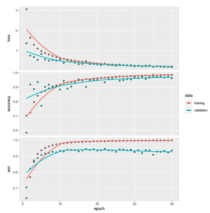
Results for the model trained with the GloVe embedding is quite similar, the model achieves a validation accuracy of 96%. The confusion matrix below shows us that only 865 reviews for restaurants that have a Michelin star are classified correctly. In this case also a few reviews of a Michelin star restaurant are not recognized as such (436 False Negatives) and quite a bit of reviews are classified as coming from a Michelin star restaurant (1.202 False Positives) but in reality are not. Overall the results of using only the GloVe word embedding for our prediction is comparable to the Word2Vec model, an F1-score of 0.51 versus 0.55. But we have more tricks up our sleeves, next we will be adding review and restaurant features to the input.
# Use model to predict probability of Michelin star on test data
glove_result <- as.data.frame(predict(model_glove, input_test_text))

# Add the real label to the dataframe
glove_result$actual  <- y_test

# From Keras we get a probability > convert to label, cut-off at 0.5
glove_result <- glove_result %>% mutate(predict = case_when(V1 > .4949 ~1, TRUE ~0)) %>% rename(probability = V1)

# Display results in a table
confusion_matrix <- table(glove_result$actual, glove_result$predict, dnn = c('actual', 'predicted'))
print(confusion_matrix)
         predicted
actual     0     1
     0 41287  1202
     1   436   865
TP <- confusion_matrix[2,2] # True Positives
FP <- confusion_matrix[1,2] # False Positives
FN <- confusion_matrix[2,1] # False Negatives
TN <- confusion_matrix[1,1] # True Negatives

#Accuracy: What % of all predictions are correct?
Accuracy = (TP+TN)/(TP+FP+FN+TN)
cat('\n Accuracy:   ', scales::percent(Accuracy),' of all Michelin/non-Michelin review predictions are correct')

#Precision: What % of predicted Michelin reviews are actually Michel*****************in reviews?
Precision = (TP)/(TP+FP)
cat('\n Precision:  ', scales::percent(Precision),' of predicted Michelin reviews are actually Michelin reviews')

#Recall/Sensitivity: What % of all actual Michelin reviews are predicted as such?
Recall = (TP)/(TP+FN)
cat('\n Recall:     ', scales::percent(Recall),' of all actual Michelin reviews are predicted as such')

#F1.Score = weighted average of Precision and Recall
F1.Score = 2*(Recall * Precision) / (Recall + Precision)
cat('\n F1 score:  ', round(F1.Score,2),' is the weighted average of Precision and Recall')
Accuracy: 96% of Michelin/non-Michelin review predictions r correct
Precision: 42% predicted Michelin reviews are real Michelin reviews
Recall: 66% of all actual Michelin reviews are predicted as such
F1 score: 0.51  is the weighted average of Precision and Recall
Predicting Michelin star restaurantreviews using word embedding and review features
Like in many analysis setups, we have the availability of both text and quantified features from the restaurant reviews. In this section we are combining both, for this we need to use the Keras Functional API. So the instructions for Keras look a bit different than before. We use a concatenate layer to combine the output from the embedding layer (containing the weights for the word embedding) and the other review features. We start with a model using the review and restaurant features and the word embedding matrix built using the Word2vec technique. If you want to know more on the usage of the Keras Functional API this post is a good introduction.
Until now my experience is that the Keras memory of earlier build models (which is connected to the Tensorflow backend) is not always cleared properly. To avoid building upon older models unintendedly, we add code to explicitly delete older session info after making slight changes. This to make sure we are building a model without any history. Also, we’ve noticed that a re-run of models might lead to a different distribution in the confusion matrix, sometimes more False Positives and sometimes more False Negatives. This is caused by the little absolute amount of reviews coming from a Michelin star restaurant in the test dataset. From now on we will not present the full confusion matrix but focus on the AUC, accuracy and plot cumulative gains charts for all models at the end of this section.
# make sure we clean all keras nodes (memory efficient & avoid re-fitting old models)
K <- backend()
K$clear_session()

# How many features are in our set?
numfeat = ncol(x_train_features)

# Since we have word embeddings AND other features, we should not use keras_model_sequential but the keras functional API. Setting up the inputs:
text_input <- layer_input(shape=c(max_length),name='text')
feature_input <- layer_input(shape=c(numfeat),name='features')

# Output from the embedding layer, using the Word2Vec embedding matrix, no new training
embedding_out <- text_input %>%
                 layer_embedding(input_dim = num_tokens+1, output_dim = word2vecdim, input_length=max_length,
                                 weights=list(word2vec_embedding), trainable=FALSE) %>%
                 layer_flatten()

# Output of both the text and features & classify with a sigmoid
outputtot <-  layer_concatenate(c(embedding_out,feature_input)) %>%
              layer_dense(units = 40, activation = "relu", kernel_initializer = "he_normal", bias_initializer = "zeros",
                          kernel_regularizer = regularizer_l2(0.05)) %>% layer_dropout(rate = 0.2) %>%
              # add a dense layer with 20 units
              layer_dense(units = 20, activation = "relu", kernel_regularizer = regularizer_l2(0.05)) %>%
              # add the classifier on top
              layer_dense(units = 1, activation = "sigmoid")

# save the setup in a model
model_word2vec_2 <- keras_model(inputs=c(text_input,feature_input),outputs=outputtot)
We stick to our rmsprop optimizer and the same loss function as before. Note that the ‘Adam’ optimizer is gaining importance (Adaptive Moment Estimation). Instead of using a fixed learning rate for the optimizer, Adam uses a rate per parameter. Within the deep learnig field it is in favor because it is very memory efficient for large models and datasets. Another option you have is to vary the rate of the loss function during training (callback_reduce_lr_on_plateau). When the validation AUC falls behind on next iterations the loss rate will be adapted (lowered), which could get you away from a plateau with suboptimal results.
model_word2vec_2 %>% compile(
  optimizer = "rmsprop",
  # we have a binary classification, a single unit sigmoid in the dense layer so binary_crossentropy
  loss = "binary_crossentropy",
  # plot the Area under the Curve against train and testset
  metrics = c("accuracy", "AUC")
)

# Use a class weights since we have very little michelin restaurants
weight = nrow(y_train) / sum(y_train)

history <- model_word2vec_2 %>% fit(
  x=list(input_train_text,as.matrix(x_train_features)),
  y=y_train,
  # maximum number of iterations
  epochs = 20,
  # how many reviews do we offer in each batch
  batch_size = 5000,
  # we have little Michelin restaurants, so we need to focus more on classifying these (set weights)
  class_weight = list("0"=1,"1"=weight),
  # check train results againts test data
  validation_data = list(list(input_test_text, as.matrix(x_test_features)), y = as.matrix(y_test))
)
loss: 0.7568 - accuracy: 0.9381 - auc: 0.9861 - val_loss: 0.4609 - val_accuracy: 0.9767 - val_auc: 0.9555
After 20 epochs the model reaches a validation Area Under the Curve of almost 96%. Adding other features to the model, that were very significant in the previous Random Forest model in the topic modeling blog, has little effect here. Before looking into results in more detail we will first run the model with the GloVe word embedding and compare performances between models.
Glove with features
Below we use the same architecture and provide the GloVe word embedding as input weights for the embedding layer.
# How many features are in our set?
numfeat = ncol(x_train_features)
# since we have word embeddings AND other features, we should not use keras_model_sequential but the keras functional API
text_input <- layer_input(shape=c(max_length),name='text')
embedding_out <- text_input %>%
layer_embedding(input_dim = num_tokens+1, output_dim = glovedim, input_length=max_length,
weights=list(embedding_matrix_glove), trainable=TRUE) %>%
layer_flatten()
feature_input <- layer_input(shape=c(numfeat),name='features')
outputtot <- layer_concatenate(c(embedding_out,feature_input)) %>%
layer_dense(units = 40, activation = "relu", kernel_initializer = "he_normal", bias_initializer = "zeros",
kernel_regularizer = regularizer_l2(0.05)) %>% layer_dropout(rate = 0.2) %>%
# add a dense layer with 20 units
layer_dense(units = 20, activation = "relu", kernel_regularizer = regularizer_l2(0.05)) %>%
# add the classifier on top
layer_dense(units = 1, activation = "sigmoid")
model_glove_2 <- keras_model(inputs=c(text_input,feature_input),outputs=outputtot)
# Network with two inputs: text and features, using the Keras Functional API
model_glove_2 %>% compile(
optimizer = "rmsprop",
# we have a binary classification, a single unit sigmoid in the dense layer so binary_crossentropy
loss = "binary_crossentropy",
# plot accuracy against train and testset
metrics = list("accuracy", "AUC")
)
# Use a class weights since we have very little michelin restaurants
weight = nrow(y_train) / sum(y_train)
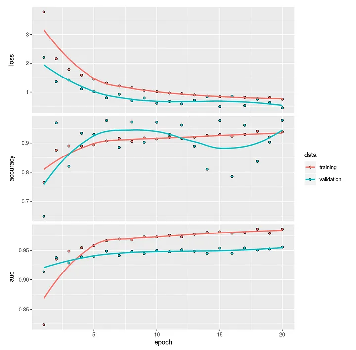
history <- model_glove_2 %>% fit(
x=list(input_train_text,as.matrix(x_train_features)),
y=y_train,
# we have little Michelin restaurants, so we need to focus more on classifying these (set weights)
class_weight = list("0"=1,"1"=weight),
# maximum number of iterations
epochs = 20,
# how many reviews do we offer in each batch
batch_size = 5000,
# callbacks = list(callback_reduce_lr_on_plateau(monitor = "val_loss", factor = 0.05)),
# check train results againts test data
validation_data = list(list(input_test_text, as.matrix(x_test_features)), y = as.matrix(y_test))
loss: 0.4429 - accuracy: 0.9559 - auc: 0.9921 - val_loss: 0.3259 - val_accuracy: 0.9613 - val_auc: 0.9479
Performance of the model using the GloVe word embedding including the reviewer and restaurant features is not better than the model without features. The AUC of almost 95% and an accuracy of 96% is about the same. So overall we do not see improvement of models when we include additional features of the review or the reviewer into the model. The word embeddings alone are capable of providing a decent model score.
Compare model performance
Time to take a closer look the performance of all our models we have made; the word embedding models versus the baseline Random Forest model using topics as input. As you might have read in our previous article, where we predicted Michelin star reviews using Topic Modeling, we are using a package called modelplotr to get more insights in the quality of the predictive models. The package provides plots which are very insightful. These plots are all based on the predicted probability instead of the ‘hard’ prediction based on a cutoff value. Let’s explore how well we can predict Michelin reviews with the models built upon Word Embedding compared to the Random Forest model using Topic Modeling.
library(modelplotr)

# For scoring of Keras models input as a list is required
input_test_textonly = list(input_test_text)
input_test_text_features = list(input_test_text,x_test_features)

# Score models based on text only and save validation predictions in dataframe
scores_and_ntiles_textonly_val <- prepare_scores_and_ntiles_keras(inputlist=list('input_test_textonly'),
                                                                  inputlist_labels=list('test data'),
                                                                  outputlists=list('y_test'),
                                                                  models = list('model_word2vec','model_glove'),
                                                                  model_labels=list('Word2Vec (NN)','GloVe (NN)'),
                                                                  ntiles = 100)

# Score models based on text and extra features and save validation predictions in dataframe
scores_and_ntiles_textfeat_val <- prepare_scores_and_ntiles_keras(inputlist=list('input_test_text_features'),
                                                                  inputlist_labels=list('test data'),
                                                                  outputlists=list('y_test'),
                                                                  models = list('model_word2vec_2','model_glove_2'),
                                                                  model_labels=list('Word2Vec + feat (NN)','GloVe + feat (NN)'),
                                                                  ntiles = 100)

# Bind all predictions in one dataset as input for Modelplotr, we do not need the ReviewRestoID here
scores_and_ntiles <- rbind(scores_and_ntiles_rf,scores_and_ntiles_textonly_val,scores_and_ntiles_textfeat_val)
str(scores_and_ntiles)
'data.frame':	321026 obs. of  7 variables:
 $ model_label  : chr  "Topic Modeling (RF)" "Topic Modeling (RF)" "Topic Modeling (RF)" "Topic Modeling (RF)" ...
 $ dataset_label: Factor w/ 2 levels "train data","test data": 1 1 1
 $ y_true       : Factor w/ 2 levels "0","1": 1 1 1 1 1 1 1 1 1 ...
 $ prob_0       : num  0.998 1 0.998 1 1 0.994 1 0.938 1 0.972 ...
 $ prob_1       : num  0.002 0 0.002 0 0 0.006 0 0.062 0 0.028 ...
 $ ntl_0        : num  48 17 45 10 33 62 3 94 21 86 ...
 $ ntl_1        : num  50 69 49 64 66 40 77 7 97 15 ...
For an introduction in how the modelplotr plots help to assess the (business) value of a predictive model, see ?modelplotr or read this. In short:
- Cumulative gains plot, helps answering the question: When we apply the model and select the best X ntiles, what percentage of the actual target class observations can we expect to target?
- Cumulative lift plot or index plot, helps you answer the question: When we apply the model and select the best X ntiles, how many times better is that than using no model at all?
- Response plot, plots the percentage of target class observations per ntile. It can be used to answer the following business question: When we apply the model and select ntile X, what is the expected percentage of target class observations in that ntile?
- Cumulative response plot, plots the cumulative percentage of target class observations up until that ntile. It helps answering the question: When we apply the model and select up until ntile X, what is the expected percentage of target class observations in the selection?
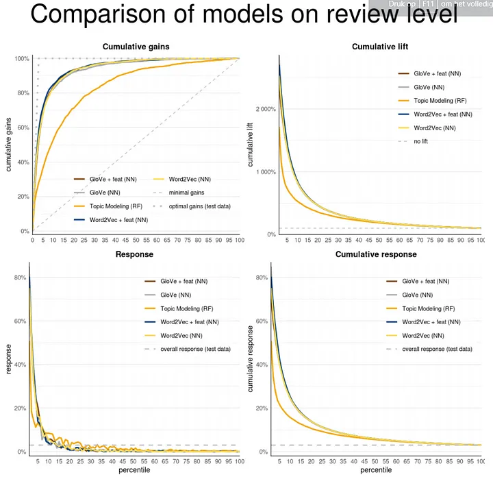
In general all models using the word embeddings clearly outperform the Random Forest model containing the results from Topic Modeling. After 5 percent of the cases with the highest probabilities the Random Forest model retrieves 36% of all positive cases (473 out of 1301), the Word2Vec model including other features retrieves 71% (930) of all cases.
# Compare models at 5th ntile
plot_input <- plotting_scope(prepared_input = scores_and_ntiles,scope="compare_models",select_dataset='test data')
plot_input %>%
 filter(ntile == 5 & dataset_label=='test data') %>%
 select(c('model_label', 'postot', 'cumpos', 'cumgain')) %>%
 arrange(desc(cumpos))
model_label              postot cumpos cumgain
1 Word2Vec + feat (NN)   1301    930 0.7148347
2           GloVe (NN)   1301    902 0.6933128
3    GloVe + feat (NN)   1301    889 0.6833205
4        Word2Vec (NN)   1301    877 0.6740968
5  Topic Modeling (RF)   1301    473 0.3635665
The plots created by the modelplotr package show the difference in performance between the word embeddings models and the topic modeling model. All models using word embedding follow the same trajectory with the Word2Vec model inclusing features (blue line) slightly better than the rest. That the Word2Vec model is somewhat better than the GloVe model on the review level is surprising since the interpretability of the GloVe embedding -at face-value- seemed better when we visualised word similarity in our previous article.
# Add a custom title
my_plot_text <- customize_plot_text(plot_input = plot_input)
my_plot_text$multiplot$plottitle <- 'Comparison of models on review level'

# Plot results on review level for all models
plot_multiplot(plot_input,
               custom_plot_text = my_plot_text,
               custom_line_colors=c("#7C3F00", "#ACACAC", "#F5A507", "#003D7C", "#FFDC51"))
As we introduced above we are most interested in the performance of the models on restaurant level. Up till now we’ve been looking at predicting on the review level whether it concerns reviews for Michelin restaurants versus reviews for non-Michelin restaurants. We aggregate our review prediction scores to the restaurant level to see how good we are in distinguishing Michelin from non-Michelin restaurants based on what texts reviewers use in reviewing the restaurants. That would mean that we can distinguish a Michelin restaurant from a non-Michelin restaurant, only looking at how visitors write about it in their reviews. On the restaurant level we calculate the mean probability of all reviews for a restaurant.
# Retrieve Random Forest Topic Model score on resto level
scores_and_ntiles_rf_val_resto <- readRDS(url('https://bhciaaablob.blob.core.windows.net/cmotionsnlpblogs/rf.topicscores.otherfeat.resto.RDS','rb'))
scores_and_ntiles_rf_val_resto$model_label <- 'Topic Modeling (RF)'

# Create scores on resto level instead of review level
scores_and_ntiles_nn_val_resto <-scores_and_ntiles %>%
                      filter(model_label!='Topic Modeling (RF)') %>% # remove topic model RF scores (we'll add the topic model rf scores on resto niveau later)
                      mutate(restoReviewId= rep(trainids$restoReviewId[trainids$train==0], 4)) %>% #add the restoReviewId to the scored data
                      mutate(restoId = as.numeric(str_extract(restoReviewId, "[^_]+"))) %>%  #restoId is part of the restoReviewId
                      mutate(y_true=as.numeric(as.character(y_true))) %>% #y_true is a factor with levels 1='0' and 2='1'
                      group_by(model_label, dataset_label, restoId) %>%
                      summarise(aant_reviews=n(), y_true=max(y_true), prob_0=mean(prob_0), prob_1=mean(prob_1)) %>%
                      group_by(model_label, dataset_label) %>%
                      arrange(-prob_0) %>%
                      mutate(ntl_0 = ntile(-prob_0,n=100), ntl_1 = 100+1-ntl_0)%>%
                      select(-c(aant_reviews)) %>%
                      ungroup()


# Bind all predictions in one dataset as input for Modelplotr
scores_and_ntiles_resto <- rbind(scores_and_ntiles_rf_val_resto,scores_and_ntiles_nn_val_resto)
On restaurant level the Random Forest model using Topics has a cumulative gain of 69% at the 5th ntile. Models using word embedding have a cumulative gain of around 90% after 5% of all cases. The Word2Vec model including features ranks the top position with a 101 retrieved restaurant out of 110. That is quite an achievement! Noteworthy also is that predictive models solely using the word embeddings already have a very high cumulative gain. Below we plot the best embedding model against the random forest topic model in modelplotr.
model_label             postot cumpos cumgain
1 Word2Vec + feat (NN)    110    101 0.9181818
2    GloVe + feat (NN)    110    100 0.9090909
3        Word2Vec (NN)    110     99 0.9000000
4           GloVe (NN)    110     98 0.8909091
5  Topic Modeling (RF)    110     76 0.6909091
plot_input_resto <- plotting_scope(prepared_input = scores_and_ntiles_resto,scope="compare_models",select_dataset='test data', select_model_label=c('Word2Vec + feat (NN)', 'Topic Modeling (RF)'))
my_plot_text$multiplot$plottitle <- 'Word embedding versus baseline model on restaurant level'
plot_multiplot(plot_input_resto,
               custom_plot_text = my_plot_text,
               custom_line_colors=c("#F5A507", "#003D7C"))

Standing on the shoulders of giants — using Transfer Learning
Transfer Learning means you use a model that was trained on another task and apply it to your own task. Within the field of deep learning usage of pre-trained models is done often because it saves a lot of computing time and resources. There are pre-trained embedding models available for natural language purposes that are trained on Wikipedia, the Google Books index of social media posts. Because these models were trained on very large corpora they have billion of sentences to learn from and contain 300k unique tokens for the English Wikipedia.
In our word embedding articles we choose to build our own embedding models as we thought this would be a great learning experience and also beneficial for the end result. How can a pre-trained model from an entirely different context perform better than a model tailored for the task it is trained for? Let’s find out if that is correct by using an externally pre-trained embedding model. For our task we will use a pre-trained model based on the Dutch Wikipedia pages. This model has 160 trained word embedding dimensions and was created by researchers for the University of Antwerp.
# Read Wikipedia embedding matrix (160 dimensions)
td = tempdir()
tf = tempfile(tmpdir=td, fileext=".tar.gz")
download.file('https://www.clips.uantwerpen.be/dutchembeddings/wikipedia-160.tar.gz', tf)
untar(file.path(tf))
Below we unpack the Wikipedia embeddings and create an embedding matrix as input for our neural network model.
# Create a list of the words in our index
word_index = tokenizer_train$word_index

# how many dimensions in our pre-trained set
wiki_pretrained_dim <- 160

# how many words
num_words <- num_tokens + 1

# read raw wikipedia embedding file
lines <- readLines(file.path("160/wikipedia-160.txt"))

# unpack those lines and seperate words with a space
wiki_embeddings_index <- new.env(hash = TRUE, parent = emptyenv())
for (i in 1:length(lines)) {
  line <- lines[[i]]
  values <- strsplit(line, " ")[[1]]
  word <- values[[1]]
  wiki_embeddings_index[[word]] <- as.double(values[-1])
}

# put results in marix format as input for Keras
wiki_prepare_embedding_matrix <- function() {
  embedding_matrix <- matrix(0L, nrow = num_words, ncol = wiki_pretrained_dim)
  embedding_names <- matrix(0L, nrow = num_words, ncol = 1)
  for (word in names(word_index)) {
    index <- word_index[[word]]
    if (index >= max_length)
      next
    embedding_vector <- wiki_embeddings_index[[word]]
    if (!is.null(embedding_vector)) {
      # words not found in embedding index will be all-zeros.
      embedding_matrix[index,] <- embedding_vector
      embedding_names[index] <- word
    }
  }
  row.names(embedding_matrix) <- embedding_names
  embedding_matrix
}

wiki_trained_embedding_matrix <- wiki_prepare_embedding_matrix()

# If you want to use this matrix yourself and don't want to download and unpack, read the file below
# wiki_trained_embedding_matrix <- readRDS(url('https://bhciaaablob.blob.core.windows.net/cmotionsnlpblogs/trained_embedding_matrix.RDS','rb'))
Below we set up our architecture in the same way we did for previous models. We insert the weights of the pre-trained Wikipedia embedding matrix into the embedding layer and prohibit any further trained for this layer.
# How many features are in our set?
numfeat = ncol(x_train_features)

# how many dimensions in our pre-trained Wikipedia dataset
pretrained_dim <- 160

# since we have word embeddings AND other features, we should not use keras_model_sequential but the keras functional API
text_input <- layer_input(shape=c(max_length),name='text')
embedding_out <- text_input %>%
                 layer_embedding(input_dim = num_tokens+1, output_dim = pretrained_dim, input_length=max_length, weights=list(wiki_trained_embedding_matrix), trainable=TRUE) %>%
                 layer_flatten()
feature_input <- layer_input(shape=c(numfeat),name='features')

outputtot <- layer_concatenate(c(embedding_out,feature_input)) %>%
  layer_dense(units = 40, activation = "relu", kernel_initializer = "he_normal", bias_initializer = "zeros", kernel_regularizer = regularizer_l2(0.1)) %>% layer_dropout(rate = 0.2) %>%
              # add a dense layer with 20 units
              layer_dense(units = 20, activation = "relu", kernel_regularizer = regularizer_l2(0.05)) %>%
              # add the classifier on top
              layer_dense(units = 1, activation = "sigmoid")

model_wiki_trained_embeddings <- keras_model(inputs=c(text_input,feature_input),outputs=outputtot)
model_wiki_trained_embeddings %>% compile(
optimizer = "rmsprop",
# we have a binary classification, a single unit sigmoid in the dense layer so binary_crossentropy
loss = "binary_crossentropy",
# plot accuracy against train and testset
metrics = list("accuracy", "AUC")
)
# Use a class weights since we have very little michelin restaurants
weight = nrow(y_train) / sum(y_train)
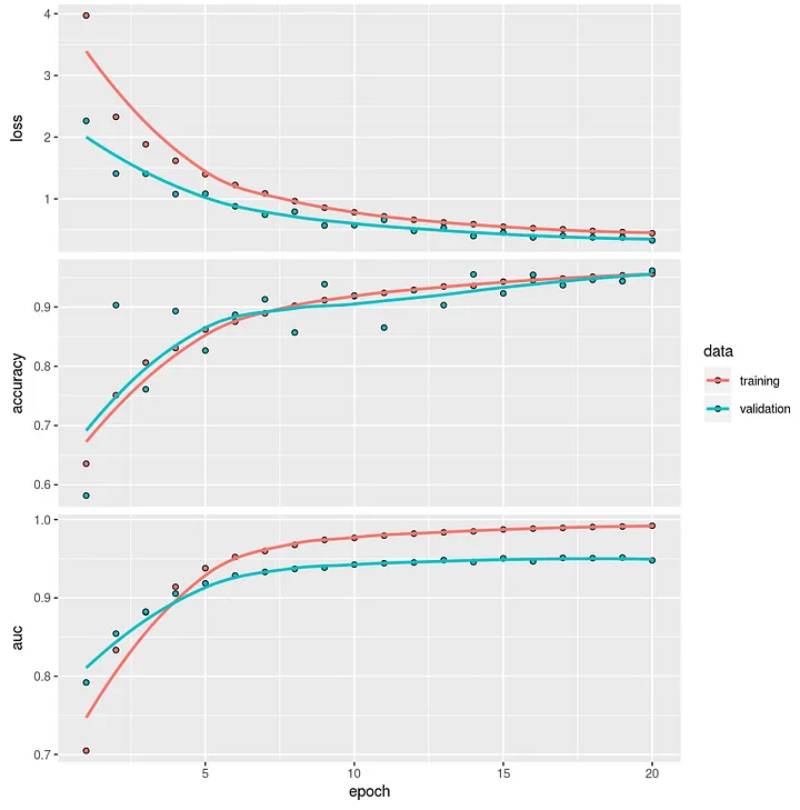
history <- model_wiki_trained_embeddings %>% fit(
x=list(input_train_text,as.matrix(x_train_features)),
y=y_train,
# we have little Michelin restaurants, so we need to focus more on classifying these (set weights)
class_weight = list("0"=1,"1"=weight),
# maximum number of iterations
epochs = 20,
# how many reviews do we offer in each batch
batch_size = 2000,
# check train results againts test data
validation_data = list(list(input_test_text, as.matrix(x_test_features)), y = as.matrix(y_test))
)
loss: 0.3390 - accuracy: 0.9676 - auc: 0.9951 - val_loss: 0.4341 - val_accuracy: 0.9744 - val_auc: 0.9317
After training 20 epochs the model reaches and AUC of 93% and an accuracy of 97%, slightly lower than previous models using custom build word embeddings.
# Prepare scores of Wikipedia Transfer Model for modelplotr
scores_and_ntiles_textfeat_wiki_val <- prepare_scores_and_ntiles_keras(inputlist=list('input_test_text_features'),
                                                                  inputlist_labels=list('test data'),
                                                                  outputlists=list('y_test'),
                                                                  models = list('model_wiki_trained_embeddings'),
                                                                  model_labels=list('Transfer Learning Wiki (NN)'),
                                                                  ntiles = 100)

# Add model scores using Wikipedia embedding to the other scores
scores_and_ntiles <- rbind(scores_and_ntiles,scores_and_ntiles_textfeat_wiki_val)

# Bring model results for Wiki Transfer Learning to restaurant level
scores_and_ntiles_wiki_val_resto <- scores_and_ntiles_textfeat_wiki_val %>%
                      mutate(restoReviewId= trainids$restoReviewId[trainids$train==0]) %>% #add the restoReviewId to the scored data
                      mutate(restoId = as.numeric(str_extract(restoReviewId, "[^_]+"))) %>%  #restoId is part of the restoReviewId
                      mutate(y_true=as.numeric(as.character(y_true))) %>% #y_true is a factor with levels 1='0' and 2='1'
                      group_by(model_label, dataset_label, restoId) %>%
                      summarise(aant_reviews=n(), y_true=max(y_true), prob_0=mean(prob_0), prob_1=mean(prob_1)) %>%
                      group_by(model_label, dataset_label) %>%
                      arrange(-prob_0) %>%
                      mutate(ntl_0 = ntile(-prob_0,n=100), ntl_1 = 100+1-ntl_0)%>%
                      select(-c(aant_reviews)) %>%
                      ungroup()


# Bind all predictions in one dataset as input for Modelplotr
scores_and_ntiles_resto <- rbind(scores_and_ntiles_resto,scores_and_ntiles_wiki_val_resto)
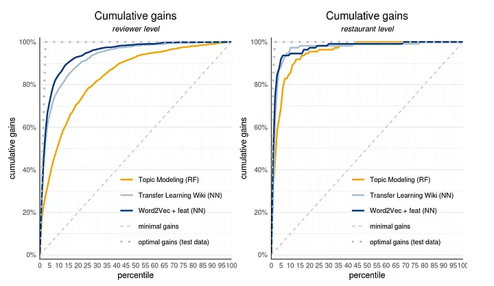
From the plots you can clearly see that the model using the pre-trained Wikipedia embedding does not have a better performance than the self trained GloVe model on the restaurant reviews dataset; both on the review level and the restaurant level. In our case using a pre-trained model does not increase performance of our downstream task.
# Show final model results on review and restaurant level side-by-side
library(gridExtra)

plot_input <- plotting_scope(prepared_input = scores_and_ntiles,scope="compare_models",select_dataset='test data',
                             select_model_label=list("Word2Vec + feat (NN)","Topic Modeling (RF)","Transfer Learning Wiki (NN)"))
my_plot_text$cumgains$plottitle <- 'Cumulative gains'
my_plot_text$cumgains$plotsubtitle <- 'reviewer level'
review_level <- plot_cumgains(plot_input, custom_plot_text = my_plot_text, custom_line_colors=c("#F5A507", "#AABED3", "#003D7C"))

plot_input_resto <- plotting_scope(prepared_input = scores_and_ntiles_resto,scope="compare_models",select_dataset='test data',
                             select_model_label=list("Word2Vec + feat (NN)","Topic Modeling (RF)","Transfer Learning Wiki (NN)"))
my_plot_text$cumgains$plotsubtitle <- 'restaurant level'
restaurant_level <- plot_cumgains(plot_input_resto, custom_plot_text = my_plot_text, custom_line_colors=c("#F5A507", "#AABED3", "#003D7C"))

# Put the results side-by-side for a comparison
options(repr.plot.width=1000, repr.plot.height=600)
grid.arrange(review_level,restaurant_level, ncol=2)
Wrapping it up
In this article we used word embeddings to predict which restaurant is more likely to receive a next Michelin star. As we’ve seen in our previous article these word embeddings are useful in capturing semantic similarities on the words in your documents. At face value the Word2Vec model seemed less promising than the GloVe model. However, in this article it became very clear that the Word2Vec embedding model and the GloVe embedding model do a far better job than the Random Forest model using topics. Both perform very well for our downstream NLP prediction task: predicting Michelin star restaurant reviews on a validation dataset. Additional reviewer and restaurant characteristics only slightly increased model performance.
From the beginning we trained the word embeddings ourselves since we thought restaurants reviews have a niche context. We introduced Transfer Learning in this article (using knowledge gained elsewhere) by applying a large scale embedding model trained on the Dutch Wikipedia Corpus. Performance of the pre-trained Wikipedia embedding model was not better than our self trained word embedding models. In our next and final article in the NLP series we will apply a state-of-the-art NLP technique know as Transformer models, more specifically the BERT variant. The Transformer models have revolutionized NLP by looking at the relevant context of words in a sequence.
This article of part of our NLP with R series. An overview of all articles within the series can be found here.
- Previous in this series: Topic Modeling for Prediction Purposes
- Next up in this series: Transformers & BERT
Do you want to do this yourself? Please feel free to download the Databricks Notebook or the R-script from out gitlab page.