
Using Topic Modeling Results to predict Michelin Stars
In a sequence of articles we compare different NLP techniques to show you how we get valuable information from unstructured text. About a year ago we gathered reviews on Dutch restaurants. We were wondering whether ‘the wisdom of the crowd’ — reviews from restaurant visitors — could be used to predict which restaurants are most likely to receive a new Michelin-star. Read this post to see how that worked out. We used topic modeling as our primary tool to extract information from the review texts and combined that with predictive modeling techniques to end up with our predictions.
We got a lot of attention with our predictions and also questions about how we did the text analysis part. To answer these questions, we explain our approach in more detail in a series of articles on NLP. But we didn’t stop exploring NLP techniques after our publication, and we also like to share insights from adding more novel NLP techniques. More specifically we will use two types of word embeddings — a classic Word2Vec model and a GLoVe embedding model — we’ll use transfer learning with pretrained word embeddings and we use BERT. We compare the added value of these advanced NLP techniques to our baseline topic model on the same dataset. By showing what we did and how we did it, we hope to guide others that are keen to use textual data for their own data science endeavours.
In a previous article, we introduced Topic Modeling and showed you how to identify topics and visualise topic model results. In this article, we use the results from our Topic Model to predict Michelin Restaurants.
Step 0: Setting up our context
First, we set up our workbook environment with the required packages to predict Michelin stars based on the topic model we’ve created.
In our blog on preparing the textual data we already briefly introduced tidyverse and tidytext. Here, we add a few other packages to the list:
- topicmodels is a package to estimate topic models with LDA and builds upon data structures created with the tm package
- randomForest package is used to train our predictive model.
- modelplotr is used to visualise the performance of the model and to compare models
# Loading packages
library(randomForest)
library(tidyverse)
library(tidytext)
library(topicmodels)
library(modelplotr)
Step 1. Load prepared data and trained topic model
In this blog, we build further on what we did in two previous blogs and we start by loading the results from that. In the datapreparation blog, we explain in detail how we preprocessed the data, resulting in the following 5 files we can use in our NLP analytics:
- reviews.csv: a csv file with original and prepared review texts — the fuel for our NLP analyses. (included key: restoreviewid, hence the unique identifier for a review)
- labels.csv: a csv file with 1 / 0 values, indicating whether the review is a review for a Michelin restaurant or not (included key: restoreviewid)
- restoid.csv: a csv file with restaurant id’s, to be able to determine which reviews belong to which restaurant (included key: restoreviewid)
- trainids.csv: a csv file with 1 / 0 values, indicating whether the review should be used for training or testing — we already split the reviews in train/test to enable reuse of the same samples for fair comparisons between techniques (included key: restoreviewid)
- features.csv: a csv file with other features regarding the reviews (included key: restoreviewid)
In the topic modeling blog we show in detail how we ended up with our 7 topics, which we want to use as features in predicting Michelin stars. This file is named:
- lda_fit_def.RDS: an R object with the chosen topic model with 7 topics
Both the preprocessed data files and the topic model file are made available to you via public blob storage so that we can load them here and you can run all code we present yourself and see how things work in more detail.
# **reviews.csv**: a csv file with review texts - the fuel for our NLP analyses.
#   (included key: restoreviewid, hence the unique identifier for a review)
reviews <- read.csv(
  file = 'https://bhciaaablob.blob.core.windows.net/cmotionsnlpblogs/reviews.csv',
  header=TRUE,stringsAsFactors=FALSE)

# **labels.csv**: a csv file with 1 / 0 values, indicating whether the review is a review
#   for a Michelin restaurant or not (included key: restoreviewid)
labels <- read.csv(
  file = 'https://bhciaaablob.blob.core.windows.net/cmotionsnlpblogs/labels.csv',
  header=TRUE,stringsAsFactors=FALSE)

# **restoid.csv**: a csv file with restaurant id's, to be able to determine which reviews
#   belong to which restaurant (included key: restoreviewid)
restoids <- read.csv(
  file = 'https://bhciaaablob.blob.core.windows.net/cmotionsnlpblogs/restoid.csv',
  header=TRUE,stringsAsFactors=FALSE)

# **trainids.csv**: a csv file with 1 / 0 values, indicating whether the review should be used
#   for training or testing - we already split the reviews in train/test to enable reuse of
#   the same samples for fair comparisons between techniques
#   (included key: restoreviewid)storage_download(cont, "blogfiles/labels.csv",overwrite =TRUE)
trainids <- read.csv(
  file = 'https://bhciaaablob.blob.core.windows.net/cmotionsnlpblogs/trainids.csv',
  header=TRUE,stringsAsFactors=FALSE)

# **features.csv**: a csv file with other features regarding the reviews
#   (included key: restoreviewid)
features <- read.csv(
  file = 'https://bhciaaablob.blob.core.windows.net/cmotionsnlpblogs/features.csv',
  header=TRUE,stringsAsFactors=FALSE)

# **lda_fit_def.RDS**: an R object with the chosen topic model with 7 topics
lda_fit_def <- readRDS(
  url('https://bhciaaablob.blob.core.windows.net/cmotionsnlpblogs/lda_fit_def.RDS','rb'))
Step 2. Generate topic probabilities per review
The reviews data contains the cleaned text and the bigrams in separate fields. We need to combine the cleaned text and bigrams and then tokenize the data — creating a dataframe with per record the review-token-combinations. Next, we can add the topic model weights to these tokens. Those weights are saved in the lda_fit_def topic model object.
To add the topic weigths to the tokens, we first need to create a dataframe that shows per token to what extent that token is associated with each topic — a higher beta means the token is more related to that topic. Creating this dataframe from the loaded topic model can easily be done using the tidytext function tidy(). As an example, below we show the topic betas for the tokens gasten (en: guests) and wijn (en: wine), whereas the token gasten has no strong associations with specific topics, the token wijn is mainly associated with topic 3.
# get topic-term beta (weight of term within topic)
topics <- tidy(lda_fit_def)

# let's see the token weights per tpoic for the token 'wijn' (EN: wine)
topics %>% filter(term %in% c('gasten','wijn')) %>% mutate_if(is.numeric, round, 5)


## A tibble: 14 x 3
#   topic term       beta
#   <dbl> <chr>     <dbl>
#       1 gasten 0.000260
#       2 gasten 0.00021
#       3 gasten 0.0014
#       4 gasten 0.0088
#       5 gasten 0.00572
#       6 gasten 0.00182
#       7 gasten 0.00188
#       1 wijn   0
#       2 wijn   0
#       3 wijn   0.180
#       4 wijn   0
#       5 wijn   0
#       6 wijn   0.00002
#       7 wijn   0.00001
Using the topic weights, we can determine to what extent each review contains tokens that are related to the 7 topics. Next, by summing all the topic weights over all the tokens in a review, and then dividing those scores by the summed weights over all topics, we get a topic probability for each topic for each review. After transposing those topic probabilities to columns, this is the input we need for our predictive model.
# get reviews, prepare the tokens, and add topic betas to tokens
# and aggregate to get topic probabilities per review
reviews_topicprobs <- reviews %>%
  # combine prepared text including bigrams
  mutate(prepared_text = paste(reviewTextClean,bigrams)) %>%
  select(restoReviewId,prepared_text) %>%
  # unnest tokens
  unnest_tokens(token, prepared_text) %>%
  # add token betas
  left_join(topics,by=c("token"="term")) %>%
  # aggregate over betas
  group_by(restoReviewId, topic) %>% summarise(beta_topic = sum(beta,na.rm=T)) %>%
  # reset beta_topic to sum to 1 over al topics
  group_by(restoReviewId) %>% mutate(prob_topic = beta_topic / sum(beta_topic,na.rm=T)) %>%
  select(-beta_topic) %>%  ungroup() %>%
  # transpose (topic probs in columns) , remove 1 column and 1 observation with NA topic scores
  pivot_wider(names_from = topic, values_from = prob_topic,names_prefix='prob_topic') %>%
  select(-prob_topicNA) %>% filter(!is.na(prob_topic1))

## show some records
#head(reviews_topicprobs)
#`summarise()` regrouping output by 'restoReviewId' (override with `.groups` argument)
## A tibble: 6 x 8
#  restoReviewId prob_topic1 prob_topic2 prob_topic3 prob_topic4 prob_topic5
#  <chr>               <dbl>       <dbl>       <dbl>       <dbl>       <dbl>
#  219267_13          0.163      0.313       0.183       0.179        0.135
#  219267_17          0.0313     0.0133      0.0167      0.0169       0.0926
#  219267_18          0.259      0.136       0.0184      0.0363       0.0568
#  219267_19          0.244      0.420       0.0477      0.120        0.130
#  219267_2           0.0315     0.00526     0.00896     0.00764      0.0406
#  219267_20          0.0242     0.573       0.0778      0.0265       0.277
## … with 2 more variables: prob_topic6 <dbl>, prob_topic7 <dbl>
Finally, let’s add the labels we gave to the topics and plot the probabilities for a sample of 50 reviews:
# topic labels
topiclabels <- c('Hospitality','Tastes & Courses','Culinary Experience & Wines','Atmosphere',
                 'Price/Quality','Plate details','Waiter & Waitress')
topiclabels <- data.frame(topic=paste0('topic',seq(1,7)),
                          topic.label=factor(topiclabels,levels=topiclabels))

# show distribution over topics for sample of reviews
reviews_topicprobs %>% sample_n(50) %>%
  pivot_longer(-restoReviewId,names_to='topic',values_to='probability') %>%
  mutate(topic=str_replace(topic,'prob_','')) %>%
  inner_join(topiclabels,by='topic') %>%
  ggplot(aes(x=restoReviewId,y=probability)) + geom_bar(aes(fill=topic.label),stat='identity')+
    coord_flip() + ggtitle('Topic probability distribution per review') + theme_minimal()  +
    theme(legend.position="right",legend.text = element_text(size=6),
          legend.title=element_blank(),plot.title = element_text(hjust = 0.5,size=12),
          axis.title = element_text(size=8),axis.text = element_text(size=8)) +
    scale_fill_brewer(palette = "Paired")
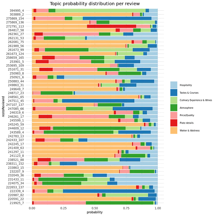
We can see, the distribution over topics is very different for different reviews. With our predictive model, we want to distinguish Michelin versus non-Michelin reviews. Do we see a difference looking at the topic probability distributions for Michelin versus non-Michelin reviews?
reviews_topicprobs %>%
  # rearrange: topic probabilities to rows
  pivot_longer(-restoReviewId,names_to='topic',values_to='probability') %>%
  mutate(topic=str_replace(topic,'prob_','')) %>%
  # add topic labels and add prediction labels
  inner_join(topiclabels,by='topic') %>% inner_join(labels,by='restoReviewId') %>%
  mutate(ReviewType=as.factor(case_when(ind_michelin==1~'Michelin',TRUE~'non-Michelin'))) %>%
  # create density plots per topic for Michelin and non-Michelin reviews
  ggplot(aes(x=probability,group=ReviewType,fill=ReviewType)) +
    geom_density(alpha=0.6) + facet_wrap(~topic.label,ncol = 4) +
    ggtitle('Topic probability distribution for Michelin / non-Michelin reviews') +
    theme_minimal()  +
    theme(legend.position=c(0.9, 0.2),legend.text = element_text(size=8),
          legend.title=element_blank(),plot.title = element_text(hjust = 0.5,size=12),
          axis.title = element_text(size=8),axis.text = element_blank()) + ylim(c(0,20))
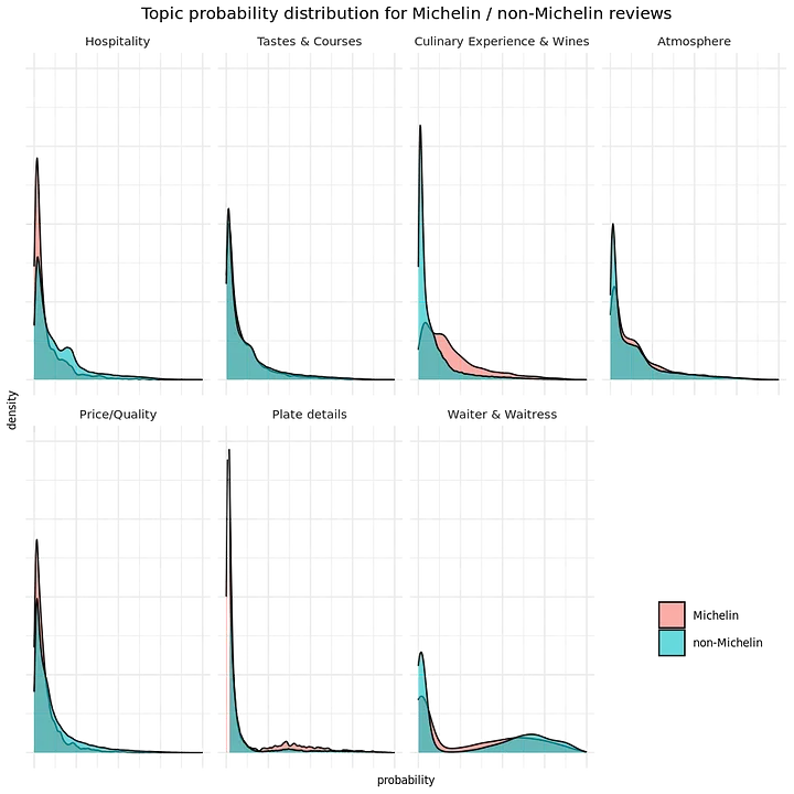
Yes, the density plots do show some differences in topic probability distributions in Michelin versus non-Michelin Reviews. For instance, in Michelin reviews there is more talk about Culinary Experience & Wines and less words spent on Hospitality compared to non-Michelin reviews. Also for other topic probabilities, we see differences. Hence, we seem to have something to work with when we want to predict Michelin reviews when using topic probabilities as predictors!
Step 3. Prepare data for predictive model
Now that we have the topic probabilities per review, we need to do some last preparations before we can estimate a predictive model predicting Michelin reviews:
- add label indicating Michelin/not-Michelin to reviews
- split in train/test set reusing previously defined train/test ids
# prepare data voor training and testing

modelinput <- reviews_topicprobs %>%
  # add label and train set indicator
  inner_join(labels,by="restoReviewId") %>% inner_join(trainids,by="restoReviewId") %>%
  # set label to factor
  mutate(ind_michelin=as.factor(ind_michelin))

train <- modelinput %>% filter(train==1) %>% select(-train)
test <- modelinput %>% filter(train!=1) %>% select(-train)

#print some rows for train
print(sample_n(train,5),width = 100)


## A tibble: 5 x 9
#  restoReviewId prob_topic1 prob_topic2 prob_topic3 prob_topic4 prob_topic5
#  <chr>               <dbl>       <dbl>       <dbl>       <dbl>       <dbl>
#  221671_14          0.349       0.195      0.0200       0.313      0.113
#  234255_127         0.279       0.0105     0.00432      0.0305     0.00600
#  246107_45          0.0624      0.417      0.0885       0.303      0.00784
#  242987_21          0.196       0.0755     0.0231       0.0453     0.630
#  249697_6           0.0441      0.251      0.0773       0.0465     0.507
#  prob_topic6 prob_topic7 ind_michelin
#        <dbl>       <dbl> <fct>
#      0.00462     0.00531 0
#      0.0190      0.650   0
#      0.0735      0.0480  0
#      0.0263      0.00335 0
#      0.0544      0.0198  0
Step 4. Predict Michelin Reviews using only topic probabilities
The train and test data contains both the labels and the topic probabilities, so we can estimate and validate a predictive model. Here, we will use a random forest model since it is fast and can easily be used with all sorts of features (we add other features in a bit).
#prepare model formula
feat_topics <- c('prob_topic1','prob_topic2','prob_topic3','prob_topic4',
                 'prob_topic5','prob_topic6','prob_topic7')
formula <- as.formula(paste('ind_michelin', paste(feat_topics, collapse=" + "), sep=" ~ "))

# estimate model (after some parameter tuning)
rf.topicscores <- randomForest(formula, data=train,ntree=500,mtry=4,min_n=50)
Feature importance: What topics help best in predicting Michelin?
Before we have a look at how good we are in predicting Michelin reviews solely based on the identified topics, let’s have a look at what are the most important topics in predicting Michelin reviews:
# get importance and add label

topiclabels <- data.frame(feature=paste0('prob_topic',seq(1,7)),
      topic_label=c('Hospitality','Tastes & Courses','Culinary Experience & Wines','Atmosphere',
              'Price/Quality','Plate details','Waiter & Waitress'))

importance(rf.topicscores) %>%
  data.frame() %>% mutate(feature=row.names(.)) %>% rename(importance=MeanDecreaseGini) %>%
  inner_join(topiclabels,by='feature') %>% select(topic_label,importance) %>%
  arrange(-importance)


#                 topic_label importance
# Culinary Experience & Wines  1020.3612
#                 Hospitality   854.4040
#               Plate details   842.7891
#                  Atmosphere   800.7580
#               Price/Quality   791.3734
#           Waiter & Waitress   767.6633
#            Tastes & Courses   764.1629
The feature importance shows that, as we expected when creating the topics as well as from our previous density plots, the topic ‘Culinary Experience & Wines’ is the most important in distinguishing between Michelin and non-Michelin Reviews.
Predictive power: How good can we predict Michelin reviews based on topics only?
Now that we know what topics matter in our prediction model, let’s evaluate how good this model is in predicting Michelin reviews. We can have a look at different statistics en plots. Often, the confusion matrix and statistics derived from that are used, so let’s start there:
# get predicted and actual values for test data
predicted <- predict(rf.topicscores,newdata=test, type="response")
actual    <- test$ind_michelin

# confusion matrix: actual vs predicted counts
confmat   <- table(actual,predicted)
print(confmat)

# derive True Positive, False Positive, False Negative and True Negative from confusion matrix
TP <- confmat[2,2]; FP <- confmat[1,2]; FN <- confmat[2,1]; TN <- confmat[1,1]

#Accuracy: What % of all predictions are correct?
Accuracy = (TP+TN)/(TP+FP+FN+TN)
cat('\n Accuracy:   ', scales::percent(Accuracy),
    ' of all Michelin/non-Michelin review predictions are correct')

#Precision: What % of predicted Michelin reviews are actually Michelin reviews?
Precision = (TP)/(TP+FP)
cat('\n Precision:  ', scales::percent(Precision),
    ' of predicted Michelin reviews are actually Michelin reviews')

#Recall(also known as Sensitivity):What % of all actual Michelin reviews are predicted as such?
Recall = (TP)/(TP+FN)
cat('\n Recall:     ', scales::percent(Recall),
    ' of all actual Michelin reviews are predicted as such')

#F1.Score = weighted average of Precision and Recall
F1.Score = 2*(Recall * Precision) / (Recall + Precision)
cat('\n F1 score:  ', round(F1.Score,2),' is the weighted average of Precision and Recall')
#      predicted
#actual     0     1
#     0 42477    12
#     1  1137   164

# Accuracy:    97%  of all Michelin/non-Michelin review predictions are correct
# Precision:   93%  of predicted Michelin reviews are actually Michelin reviews
# Recall:      13%  of all actual Michelin reviews are predicted as such
# F1 score:   0.22  is the weighted average of Precision and Recall
From the statistics above we can already conclude that, based on solely the topic probabilities, we are able to predict Michelin reviews quite good! The accuracy is very high, but this was to be expected, since only 3% of all reviews are Michelin reviews; predicting 100% as non-Michelin would also result in a 97% accuracy. This is however not the case since the model does predict 176 reviews to be Michelin reviews. The precision is 93%, hence of all the predicted Michelin reviews, 93% are in fact Michelin reviews. The recall seems somewhat low: 13% hence of all actual Michelin Reviews only 13% is predicted to be a Michelin review. But this might be due to the cutoff value used to translate the predicted probability into the prediction, by default the cutoff is a probability of 50%.
To get more insights the quality and ways to use a predictive model, some additional plots are often very insightful. These plots are all based on the predicted probability instead of the ‘hard’ 1/0 prediction based on a cutoff value. Let’s explore how well we can predict Michelin reviews with our model with only our topic scores as features with the package modelplotr:
# prepare data for modelplotr plots
scores_and_ntiles1 <- prepare_scores_and_ntiles(datasets=list("train","test"),
                                   dataset_labels = list("train data","test data"),
                                   models = list("rf.topicscores"),
                                   model_labels = list("Random Forest - Topic Modeling"),
                                   target_column="ind_michelin",
                                   ntiles = 100)
plot_input <- plotting_scope(prepared_input = scores_and_ntiles1,scope = 'no_comparison')

# plot 4 modeplotr plots together
plot_multiplot(data = plot_input)
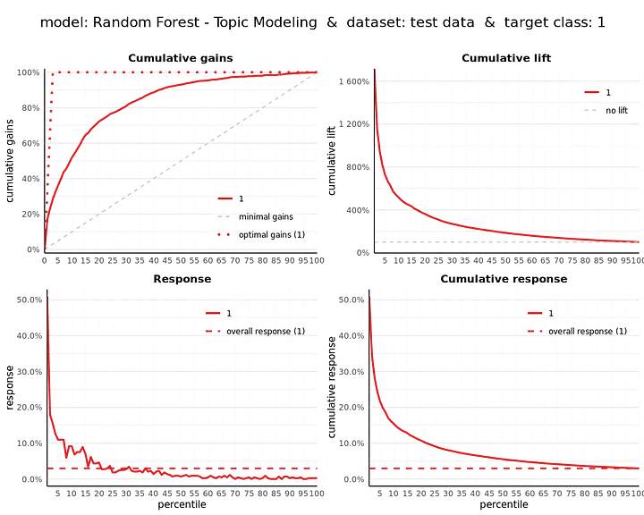
For an introduction in these how these plots help to assess the (business) value of a predictive model, see ?modelplotr or read this. In short:
- Cumulative gains plot, helps answering the question: When we apply the model and select the best X ntiles, what percentage of the actual target class observations can we expect to target?
- Cumulative lift plot or index plot, helps you answer the question: When we apply the model and select the best X ntiles, how many times better is that than using no model at all?
- Response plot, plots the percentage of target class observations per ntile. It can be used to answer the following business question: When we apply the model and select ntile X, what is the expected percentage of target class observations in that ntile?
- Cumulative response plot, plots the cumulative percentage of target class observations up until that ntile. It helps answering the question: When we apply the model and select up until ntile X, what is the expected percentage of target class observations in the selection?
From our Michelin prediction model based on the topic score features only, we see that the top 1% of all reviews with the highest probability, consist for more than 50% of actual Michelin reviews, where in total only about 3% of all reviews are Michelin reviews.
Since these plots show in more detail how good predictive models are, we will show these plots again later on when we want to compare the quality of different Michelin prediction models. First, after adding other features and in later blogs when we use other NLP techniques to get most out of the textual review data in predicting Michelin reviews.
Extra: Evaluate predictions on the restaurant level (instead of the review level)
You might question here: As your goal is to predict Michelin restaurants based on reviews, why are you looking at how good your predictions are at the review level? Good point, sport! 🙂 We chose to build our predictive models on the review level and not on the restaurant level because we don’t want to loose too much information. To build restaurant level models, we first would have to aggregate topic scores to the restaurant level, taking mean or max scores. Also, we would end up having a very limited number of observations to build models on. We can however evaluate to what extent the review-level models can be used to point out Michelin stars on the restaurant level. To do so, let’s aggregate our review scores to the restaurant level and see how good we are then in distinguishing Michelin from non-Michelin restaurants based on what texts reviewers use in reviewing the restaurants. We’ll use the average Michelin probability over all available test reviews to come up with a restaurant Michelin probability.
# prepare data
resto_scores_and_ntiles_rf <- test %>%
   # the restaurant id is the first part of the restoReviewId, before the underscore
   mutate(model_label= as.factor('random forest (topics only)'),
           dataset_label = as.factor('test data'),
           prob_0 = predict(newdata=.,object=rf.topicscores,type='prob')[,1],
           prob_1 = predict(newdata=.,object=rf.topicscores,type='prob')[,2],
           y_true=as.factor(ind_michelin),
           restoId = str_extract(restoReviewId, "[^_]+")
          ) %>%
   group_by(model_label,
            dataset_label,
            y_true,
            restoId) %>%
   summarise(prob_0=mean(prob_0),
             prob_1=mean(prob_1)) %>%
    ungroup() %>%
    arrange(-prob_0) %>%
    mutate(ntl_0 = ntile(n=100),
           ntl_1 = 101-ntl_0)

# show some records
resto_scores_and_ntiles_rf %>% sample_n(10)


## A tibble: 10 x 8
# model_label                 dataset_label y_true restoId prob_0 prob_1 ntl_0 ntl_1
# <fct>                       <fct>         <fct>  <chr>    <dbl>  <dbl> <int> <dbl>
# random forest (topics only) test data     0      222885   0.962 0.038     77    24
# random forest (topics only) test data     0      253137   0.999 0.001     14    87
# random forest (topics only) test data     0      243769   0.956 0.044     81    20
# random forest (topics only) test data     0      253013   0.986 0.0145    53    48
# random forest (topics only) test data     0      250559   0.961 0.039     78    23
# random forest (topics only) test data     0      259157   0.972 0.0280    70    31
# random forest (topics only) test data     0      239563   0.998 0.002     18    83
# random forest (topics only) test data     0      221403   0.97  0.03      72    29
# random forest (topics only) test data     0      238605   0.998 0.002     18    83
# random forest (topics only) test data     0      236957   1     0          4    97
# get predicted and actual values for test data
predicted <- case_when(resto_scores_and_ntiles_rf$prob_1>=0.5~1,TRUE~0)
actual    <- resto_scores_and_ntiles_rf$y_true

# confusion matrix: actual vs predicted counts
confmat   <- table(actual,predicted)
print(confmat)

# derive True Positive, False Positive, False Negative and True Negative from confusion matrix
TP <- confmat[2,2]; FP <- confmat[1,2]; FN <- confmat[2,1]; TN <- confmat[1,1]

#Accuracy: What % of all predictions are correct?
Accuracy = (TP+TN)/(TP+FP+FN+TN)
cat('\n Accuracy:   ', scales::percent(Accuracy),
    ' of all Michelin/non-Michelin restaurant predictions are correct')

#Precision: What % of predicted Michelin reviews are actually Michelin reviews?
Precision = (TP)/(TP+FP)
cat('\n Precision:  ', scales::percent(Precision),
    ' of predicted Michelin restaurants are actually Michelin restaurants')

#Recall: What % of all actual Michelin reviews are predicted as such?
Recall = (TP)/(TP+FN)
cat('\n Recall:     ', scales::percent(Recall),
    ' of all actual Michelin reviews are predicted as such')

#F1.Score = weighted average of Precision and Recall
F1.Score = 2*(Recall * Precision) / (Recall + Precision)
cat('\n F1 score:  ', round(F1.Score,2),' is the weighted average of Precision and Recall')

#      predicted
#actual    0    1
#     0 9323    0
#     1  105    5

# Accuracy:    99%  of all Michelin/non-Michelin restaurant predictions are correct
# Precision:   100%  of predicted Michelin restaurants are actually Michelin restaurants
# Recall:      5%  of all actual Michelin reviews are predicted as such
# F1 score:   0.09  is the weighted average of Precision and Recall
On the restaurant level, we can see that only 5 restaurants in the unseen test data have an average model probability over 50% and are therefore predicted as being a Michelin restaurant. However all of these 5 restaurants in fact are Michelin restaurants, hence our model based on topic model scores only has a Precision of 100%! There are in total 110 Michelin restaurants in our data though, hence recall (at a 50% cutoff) is only 5% and F1 Score is therefore low. Our modelplotr plots give more insights in the performance of our model on the restaurant level over the whole distribution of model probabilities:
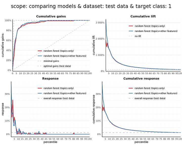
# plotting the modelplotr plots:
plot_input <- plotting_scope(prepared_input = resto_scores_and_ntiles_rf)
plot_multiplot()
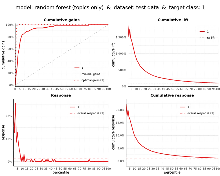
These plots show that we’ve created a model to predict Michelin star reviews — solely based on the review texts — that is quite good in predicting Michelin restaurants. Often, you have other, structured data as features available aside from the textual data. Obviously, best is to use all valuable information we have! What would happen if we would add some more features to our model?
Step 5. Predict Michelin Reviews using topic probabilities and other features
Let’s add the other features we have available about the reviews now, to see if we can further improve our prediction of Michelin reviews. In our data preparation blog we briefly discussed the other information we have available for each restaurant review and cleaned some of those features. Here, we read those and add them as predictors to predict Michelin reviews. What do we add?
- Three features are average restaurant-level scores for the restaurant over all historic reviews for Value for Price, Noise level and Waiting time;
- Reviewer Fame is a classification of the reviewer into 4 experience levels (lowest level: Proever, 2nd: Fijnproever, 3rd: Expertproever, highest: Meesterproever);
- The reviewer also evaluates and scores the Ambiance and the Service of the restaurant during the review;
- In data preparation, we calculate the total length of the review in number of characters.
- Based on pretrained international sentiment lexicons created by Data Science Lab we’ve calculated a standardized sentiment score per review. More details in our data preparation blog.
We explicitly excluded the overall score and score for the food as extra features, since we expect to be able to cover that with our NLP endeavours.
# read data

# **features.csv**: a csv file with other features regarding the reviews
#  (included key: restoreviewid)
features <- read.csv(
  file = 'https://bhciaaablob.blob.core.windows.net/cmotionsnlpblogs/features.csv',
  header=TRUE,stringsAsFactors=FALSE) %>%
  select(restoReviewId,valueForPriceScore,noiseLevelScore,waitingTimeScore,reviewerFame,
         reviewScoreService,reviewScoreAmbiance,reviewTextLength,sentiment_standardized) %>%
  mutate(reviewerFame=as.factor(reviewerFame))

str(features)
#'data.frame':	366784 obs. of  9 variables:
# $ restoReviewId         : chr  "255757_1" "255757_2" "255757_3" "255757_4" ...
# $ valueForPriceScore    : int  0 0 0 0 0 0 0 0 0 0 ...
# $ noiseLevelScore       : int  0 0 0 0 0 0 0 0 0 0 ...
# $ waitingTimeScore      : int  0 0 0 0 0 0 0 0 0 0 ...
# $ reviewerFame          : Factor w/ 5 levels "","Expertproever",..: 3 3 4 5 5 3 5 3 4 5 ...
# $ reviewScoreService    : int  8 10 6 2 2 8 8 10 10 8 ...
# $ reviewScoreAmbiance   : int  8 10 8 4 6 8 6 8 10 2 ...
# $ reviewTextLength      : int  367 278 176 811 442 16 465 146 353 291 ...
# $ sentiment_standardized: num  0.333 0.4 -0.25 -0.1 -0.818 ...
Now, let’s train a model to predict Michelin reviews using both the topic model scores and the other review characteristics as features. This is a nice example of how you can use both NLP outcomes and more conventional numeric and categorical features in one model. First, we add the features to the model input data and redo the train/test split. Then, we specify the new formula and train our extended rf.topicscores.otherfeat model. When it’s optimized, we can see to what extent the other features help in predicting Michelin reviews, by looking at feature importance and the predictive power of the model.
# add features and prepare data voor training and testing

modelinput <- reviews_topicprobs %>%
  # add label and train set indicator
  inner_join(labels,by="restoReviewId") %>% inner_join(trainids,by="restoReviewId")  %>%
  # set label to factor
  mutate(ind_michelin=as.factor(ind_michelin)) %>%
  # add extra features
  inner_join(features,by="restoReviewId")

train <- modelinput %>% filter(train==1)
test <- modelinput %>% filter(train!=1)

#prepare model formula
feat_topics <- c('prob_topic1','prob_topic2','prob_topic3','prob_topic4',
                 'prob_topic5','prob_topic6','prob_topic7')
feat_other <- c('valueForPriceScore','noiseLevelScore','waitingTimeScore','reviewerFame',
    'reviewScoreService','reviewScoreAmbiance','reviewTextLength','sentiment_standardized')
formula <- as.formula(
  paste('ind_michelin',paste(c(feat_topics,feat_other),collapse=" + "),sep=" ~ "))

# estimate model (after some parameter tuning)
rf.topicscores.otherfeat <- randomForest(formula, data=train,ntree=500,mtry=4,min_n=50)
Interestingly, the feature importance shows that the topic probabilities are much more important features when predicting Michelin reviews compared to the added features. Our hard work in discovering and labeling the topics seems to pay off! Also interesting to see is that the total review length helps in predicting Michelin reviews and that the sentiment score also is of value here. The overall restaurant scores (value for price, noise level and waiting time) as well as the review specific scores on Service and Ambiance only contribute marginally in predicting Michelin reviews.
# get importance and add label

importance(rf.topicscores.otherfeat) %>% data.frame() %>% mutate(feature=row.names(.)) %>%
  rename(importance=MeanDecreaseGini) %>%
  select(feature,importance) %>% arrange(-importance)


#                 feature importance
#             prob_topic3   740.6574
#        reviewTextLength   622.6494
#             prob_topic1   613.1067
#             prob_topic6   541.0968
#             prob_topic4   514.4275
#             prob_topic2   506.9077
#             prob_topic5   506.8417
#             prob_topic7   484.9836
#  sentiment_standardized   397.5924
#     reviewScoreAmbiance   176.6893
#      reviewScoreService   163.3590
#            reviewerFame   162.6073
#         noiseLevelScore   155.8718
#      valueForPriceScore   152.8744
#        waitingTimeScore   111.7827
Did we improve our model? Let’s have a look at the same statistics and plots as before, first on the review level and next on the restaurant level.
#      predicted
#actual     0     1
#     0 42473    16
#     1  1120   181

# Accuracy:    97%  of all Michelin/non-Michelin review predictions are correct
# Precision:   92%  of predicted Michelin reviews are actually Michelin reviews
# Recall:      14%  of all actual Michelin reviews are predicted as such
# F1 score:   0.24  is the weighted average of Precision and Recall
From the confusion matrix and related statistics, we see a small increase in performance. The recall and F1 score slightly go up. Also, from the modelplotr plots we see that we need to select less reviews to have a higher portion of actual Michelin reviews (cumulative gains) and that we are more than 20 times better (2000%) than random guessing in the top 1% according to our model (cumulative lift).
And what is the impact if we want to point out Michelin restaurants based on our review predictions? Did adding extra features improve that as well?
# prepare data
resto_scores_and_ntiles_rf2 <- test %>%
# the restaurant id is the first part of the restoReviewId, before the underscore
mutate(model_label= as.factor('random forest (topics+other features)'),
dataset_label = as.factor('test data'),
prob_0 = predict(newdata=.,object=rf.topicscores.otherfeat,type='prob')[,1],
prob_1 = predict(newdata=.,object=rf.topicscores.otherfeat,type='prob')[,2],
y_true=as.factor(ind_michelin),
restoId = str_extract(restoReviewId, "[^_]+")
) %>%
group_by(model_label,
dataset_label,
y_true,
restoId) %>%
summarise(prob_0=mean(prob_0),
prob_1=mean(prob_1)) %>%
ungroup() %>%
arrange(-prob_0) %>%
mutate(ntl_0 = ntile(n=100),
ntl_1 = 101-ntl_0)
# get predicted and actual values for test data
predicted <- case_when(resto_scores_and_ntiles_rf2$prob_1>=0.5~1,TRUE~0)
actual <- resto_scores_and_ntiles_rf2$y_true
# confusion matrix: actual vs predicted counts
confmat <- table(actual,predicted)
print(confmat)
# derive True Positive, False Positive, False Negative and True Negative from confusion matrix
TP <- confmat[2,2]; FP <- confmat[1,2]; FN <- confmat[2,1]; TN <- confmat[1,1]
#Accuracy: What % of all predictions are correct?
Accuracy = (TP+TN)/(TP+FP+FN+TN)
cat('\n Accuracy: ', scales::percent(Accuracy),
' of all Michelin/non-Michelin restaurant predictions are correct')
#Precision: What % of predicted Michelin reviews are actually Michelin reviews?
Precision = (TP)/(TP+FP)
cat('\n Precision: ', scales::percent(Precision),
' of predicted Michelin restaurants are actually Michelin restaurants')
#Recall: What % of all actual Michelin reviews are predicted as such?
Recall = (TP)/(TP+FN)
cat('\n Recall: ', scales::percent(Recall),
' of all actual Michelin reviews are predicted as such')
#F1.Score = weighted average of Precision and Recall
F1.Score = 2*(Recall * Precision) / (Recall + Precision)
cat('\n F1 score: ', round(F1.Score,2),' is the weighted average of Precision and Recall')
# predicted
#actual 0 1
# 0 9323 0
# 1 105 5
# Accuracy: 99% of all Michelin/non-Michelin restaurant predictions are correct
# Precision: 100% of predicted Michelin restaurants are actually Michelin restaurants
# Recall: 5% of all actual Michelin reviews are predicted as such
# F1 score: 0.09 is the weighted average of Precision and Recall
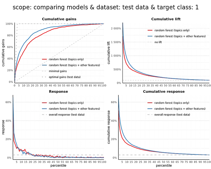
# plotting the modelplotr plots:
plot_input <- plotting_scope(prepared_input =
rbind(resto_scores_and_ntiles_rf,resto_scores_and_ntiles_rf2),scope = 'compare_models')
plot_multiplot()
Our predictions on the restaurant level improved marginally, as we can see from the statistics and plots above. The statistics, based on a 50% cutoff value, do not show any increase compared to the model based on topic scores only. If we look at the plots, we do see that the model ranks the restaurants slightly better when taking the other characteristics into account.
You might wonder: Based on the insights from the statistics and plots, do we need to change the cutoff of 50%? If this is relevant, depends on your use case. Often, the resulting rankings of scored cases — highest rank for highest model probability — is of most value to use, for instance in a campaign selection. The percentiles in the modelplotr plots are based on that ranking. You could also search for an optimal cutoff value, balancing precision and recall, to get more informative confrontation matrix and statistics, but we won’t do that here since it’s not our main interest here.
Predicting Michelin with Topic Model results — wrapping it up
In this notebook, we took the topic model results from our earlier blog on Topic Modeling and used them as features in a downstream task: predicting Michelin reviews. Although predicting Michelin reviews might not seem to have a real business value, it can easily be translated into something that does represent such value: Predicting customer behavior such as a purchase, a contract cancellation or a complaint.
Furthermore, we combined the textual features with other features, such as numeric scores and categorical features. It’s also easy to imagine how this translates to other contexts, where you often have other information available on top of the textual data. Combining those sources is most likely to result in best predictions, as we also see here.
Looking forward
In this and the earlier blog, we’ve used topic modeling to translate unstructured text into something structured we can use in downstream tasks. In recent years, many other NLP techniques have gained popularity, all with their own benefits and specifics. In our other blogs, we will use some of these techniques, such as word embeddings (Word2Vec, Glove) and BERT to see how those can be applied. And to evaluate: Will this further improve our prediction of Michelin stars?
This article is of part of our NLP with R series. An overview of all articles within the series can be found here.
- Previous in this series: Word Embedding
- Next up in this series: Using Word Embedding models for Prediction Purposes
Do you want to do this yourself? Please feel free to download the Databricks Notebook or the R-script from out gitlab page.