Training Word Embedding models and visualize results
In a sequence of articles we compare different NLP techniques to show you how we get valuable information from unstructured text. About a year ago we gathered reviews on Dutch restaurants. We were wondering whether ‘the wisdom of the crowd’ — reviews from restaurant visitors — could be used to predict which restaurants are most likely to receive a new Michelin-star. Read this post to see how that worked out. We used topic modeling as our primary tool to extract information from the review texts and combined that with predictive modeling techniques to end up with our predictions.
We got a lot of attention with our predictions and also questions about how we did the text analysis part. To answer these questions, we explain our approach in more detail in a series of articles on NLP. We didn’t stop exploring NLP techniques after our publication, and we also like to share insights from adding more novel NLP techniques. More specifically we will use two types of word embeddings — a classic Word2Vec model and a GLoVe embedding model — we’ll use transfer learning with pretrained word embeddings and we use BERT. We compare the added value of these advanced NLP techniques to our baseline topic model on the same dataset. By showing what we did and how we did it, we hope to guide others that are keen to use textual data for their own data science endeavors.
In our previous article we used topic-modeling as our primary tool to extract information from the review texts. In an upcoming article we will combine those topic modeling outcomes with predictive modeling techniques to end up with our predictions.
In this article we introduce Word Embedding and show you how a classic Word2Vec model is trained, how a GloVe model is trained, how to interprete results and finally visualize word embedding results.
Word embeddings: what is it?
In short: word embeddings are vector representations of a particular word. Word embeddings are a representation of text where words that have the same meaning have a similar representation. It is used to capture something about the meaning of words you have available, in our case restaurant reviews, in a dense representation. The result is a coordinate system where related words are placed closer together. We are going to use two different word embedding techniques on data we gathered on restaurant reviews.
This image, taken from the excellent blogs by J. Alammar The Illustrated Word2vec, provides some guidance. Below in the colored rows are 50 word embedding dimensions trained on Wikipedia data. Every word has it’s own unique encoding. The first 7 words are all human-based, their dimensions look alike and have similar colors in this illustration. On the bottom you see the encoding for water which is quite different. Of course we do not know the exact meaning of each dimension, but you might see a dimension that could encode for youth based on the similarity for boy and girl. Or a dimension that encodes for royalty with similarities for queen and king.
Sources:
Efficient Estimation of Word Representations in Vector Space by Tomas Mikolov
The illustrated word2vec by Jay Jalammar
Word2Vec Tutorial — The Skip-Gram Model by Chris McCormick
Setting up our context
In this blog we will construct Deep Learning models using the Keras framework. For an excellent introduction on building these models read Deep Learning with R written by François Chollet and and J. J. Allaire. Below we enable our workbook with the required packages and data to build our word embedding models and visualize results. In our blog on preparing the textual data we already briefly introduced tidyverse and tidytext. Here, we add a few other packages to the list:
- text2vec a very memory efficient package used for text analysis. We use is here for the native GloVe support to build our model;
- keras a popular package for building neural networks, a user friendly interface connected to the Tensorflow back-end;
- uwot is the R implementation of UMAP, a general purpose dimensionality reduction algorithm which is useful here to visualize the word embeddings.
Load preprocessed data
Before we start building a word embedding we need some prepared textual data. Proper data preparation takes most of your time and is very decisive for the quality of the analysis results you end up with. In a previous blog, we explain in detail how we preprocessed the data. We will use the following 4 files for our word embeddings:
- reviews.csv: a csv file with review texts — the fuel for our NLP analyses. (included key: restoreviewid, hence the unique identifier for a review)
- labels.csv: a csv file with 1 / 0 values, indicating whether the review is a review for a Michelin restaurant or not (included key: restoreviewid)
- restoid.csv: a csv file with restaurant id’s, to be able to determine which reviews belong to which restaurant (included key: restoreviewid)
- trainids.csv: a csv file with 1 / 0 values, indicating whether the review should be used for training or testing — we already split the reviews in train/test to enable reuse of the same samples for fair comparisons between techniques (included key: restoreviewid)
These files with the cleaned and relevant data for NLP techniques are made available to you via public blob storage. Learning by doing works best for most of us, so with the data available you are able to run all code we present yourself and see how things work out in more detail.
# Read data files from public blob storage

# **reviews.csv**: a csv file with review texts - the fuel for our NLP analyses. (included key: restoreviewid, hence the unique identifier for a review)
reviews <- read.csv(file = 'https://bhciaaablob.blob.core.windows.net/cmotionsnlpblogs/reviews.csv',header=TRUE,stringsAsFactors=FALSE)

# **labels.csv**: a csv file with 1 / 0 values, indicating whether the review is a review for a Michelin restaurant or not (included key: restoreviewid)
labels <- read.csv(file = 'https://bhciaaablob.blob.core.windows.net/cmotionsnlpblogs/labels.csv',header=TRUE,stringsAsFactors=FALSE)

# **restoid.csv**: a csv file with restaurant id's, to be able to determine which reviews belong to which restaurant (included key: restoreviewid)
restoids <- read.csv(file = 'https://bhciaaablob.blob.core.windows.net/cmotionsnlpblogs/restoid.csv',header=TRUE,stringsAsFactors=FALSE)

# **trainids.csv**: a csv file with 1 / 0 values, indicating whether the review should be used for training or testing - we already split the reviews in train/test to enable reuse of the same samples for fair comparisons between techniques (included key: restoreviewid)storage_download(cont, "blogfiles/labels.csv",overwrite =TRUE)
trainids <- read.csv(file = 'https://bhciaaablob.blob.core.windows.net/cmotionsnlpblogs/trainids.csv',header=TRUE,stringsAsFactors=FALSE)
Using a Word2Vec word embedding
In general there are two ways to obtain a word embedding. First you can learn the word embeddings yourself together with the challenge at hand: modeling which restaurant receives a Michelin star. In one model you both train the word embeddings as well as the parameters for the predictive model. You start with random word vectors and then learn the best fitting word vectors, guided by the predictive task at hand. Word embeddings are often trained using a Neural Network architecture. We will explain how this works in the next section. Another option is to use an already trained set of word embeddings from a different task, so-called pretrained word embeddings. There are many pretrained models available for a variety of languages. However, these models are usually trained on general datasets such as Wikipedia, the Google Books index or Social Media posts.
In this example we will train our own word embedding model for Dutch restaurant reviews. The result should reflect the semantic relationships between the words in this specific case. Whether we are successful at achieving proper word embeddings can be assessed by reviewing the geometrical distance between word vectors. You would expect that word that are similar, i.e. “frog” and “water”, have a smaller geometric distance than words that are not so similar in human language, i.e. “laptop” and “strawberry”. Further, the real value of the embeddings will show using downstream tasks where we use the knowledge gained on word embedding in predicting which restaurant is likely to receive a next Michelin star. This is something we will do in a forthcoming article, here we focus on the embeddings themselves.
Let’s see what is in our cleaned review text and decide how many words we are going to allow into the neural network for each review. Remember than we did a lot of cleaning already: lower case setting, remove punctuation, stop words and reviews with a low word count. As you can see below many reviews are shorter than 50 words. Based on this graph we decide to cut the number of allowed words at 150.
## divide reviewtext into separate words
reviews_tokens <- reviews %>%
    select(restoReviewId, reviewTextClean) %>%
    unnest_tokens(word, reviewTextClean)

## count the number of words per review and plot results
reviews_tokens %>%
group_by(restoReviewId) %>% summarise(n_tokens = n()) %>%
mutate(n_tokens_binned = cut(n_tokens, breaks = c(0,seq(10,300,10),Inf))) %>%
group_by(n_tokens_binned) %>% summarise(n_reviews = n()) %>%

## pass result to ggplot
ggplot(aes(x=n_tokens_binned,y=n_reviews)) +
geom_bar(stat='identity',fill='green') +
theme_minimal() +
theme(axis.text.x = element_text(angle = 45, hjust=1)) +
geom_text(size=2, aes(label=n_reviews), position=position_dodge(width=0.9), vjust=-0.25)
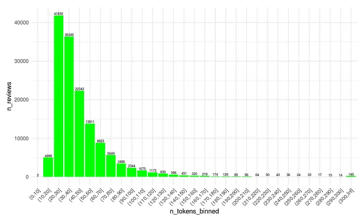
In the topic modeling blog we already showed that many words in de review corpus appear only once or twice. These words are unlikely to have a strong relation with other word in the review for embedding purposes. In the build-up of our neural network we will only use words that have a frequency of 5 or more in total. With the current collection that comes down to 37.520 unique words.
reviews_tokens %>%
group_by(word) %>% summarize(word_freq=n()) %>%
mutate(min_5_freq = case_when(word_freq<5~'token frequency: <5',TRUE~'token frequency: >=5')) %>%
group_by(min_5_freq) %>% summarise(n_tokens = n()) %>% mutate(pct_tokens = n_tokens / sum(n_tokens))
# A tibble: 2 x 3
  min_5_freq           n_tokens pct_tokens
  <chr>                   <int>      <dbl>
1 token frequency: <5    119296      0.761
2 token frequency: >=5    37520      0.239
We remove all words from the cleaned review text so they appear at least 5 times in the entire corpus. After doing so we shape the tokens back to its original form.
reviews_new <- reviews_tokens %>%
          group_by(word) %>%
          mutate(token_freq=n()) %>%
          filter(token_freq>=5) %>%
          group_by(restoReviewId) %>%
          summarise(reviewTextClean = str_c(word, collapse = " "))
Before we go any further we will split our files into train and test datasets. This way we ensure not only that we avoid overfitting but also that results are comparable with other models on the same data. All the models we build in this blog series use the same train and test IDs.
# split reviews and labels into train and test
x_train <- trainids %>% left_join(y=reviews_new, by= "restoReviewId", match = "all") %>%
filter(train == 1) %>% select(reviewTextClean) %>% pull()
x_test <- trainids %>% left_join(y=reviews_new, by= "restoReviewId", match = "all") %>%
filter(train == 0) %>% select(reviewTextClean) %>% pull()
y_train <- trainids %>% left_join(y=labels, by= "restoReviewId", match = "all") %>%
filter(train == 1) %>% select(ind_michelin) %>% pull() %>% as.array()
y_test <- trainids %>% left_join(y=labels, by= "restoReviewId", match = "all") %>%
filter(train == 0) %>% select(ind_michelin) %>% pull() %>% as.array()
Number of Michelin restaurants in train reviews: 3012 (2.1% of reviews)
Number of Michelin restaurants in test reviews: 1301 (0.9% of reviews)
Neural networks 101
Let’s talk about neural networks, they are an important ingredient for word embeddings. The basics:
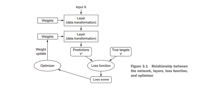
- A neural network consist of layers; combined these layers form the neural network
- The network has input data (x) and output data or targets (y)
- Between the input and the output layer, there can be one or more hidden layers of connected nodes. The architecture of the model can be simple to complex, depending on the number of hidden layers, nodes and connections between nodes.
- Within the network a loss function is calculated: the difference between the predicted target and the actual target. The loss function is used as a feedback signal for learning.
- Lastly, the network has a optimizer which determines how the network will be updated (the weights get a new value) based upon the value of the loss function.
This figure, taken from the excellent work of François Chollet and and J. J. Allaire Deep Learning with R, says it all.
When we want to use a neural network to train word embeddings on our restaurant review data, we need to convert the tokens into integers so that the neural network can take the data as an input; you cannot feed text directly into a neural network. In neural network terms we need a 2 dimensional tensor with reviews (samples) and word vectors (features). Remember that this requires the input features to be of the same length. Below we will vectorize our text, create an index and use padding (add zeros) to create equal sizes.
# maximum number of words for a review
max_length <- 150

# Vectorize the tokens, each token will receive a unique integer, the index of that token in a dictionary.
# Remember, we already restricted the corpus to 37.520 unique words.
tokenizer_train <- text_tokenizer() %>% fit_text_tokenizer(x_train)
tokenizer_test <- text_tokenizer() %>% fit_text_tokenizer(x_test)

# and put these integers into a sequence
sequences_train <- texts_to_sequences(tokenizer_train, x_train)
sequences_test <- texts_to_sequences(tokenizer_train, x_test)

# and make sure that every sequence has the same length (Keras requirement)
input_train <- pad_sequences(sequences_train, maxlen = max_length)
input_test <- pad_sequences(sequences_test, maxlen = max_length)

# show an example from the created index (word and vector)
tokenizer_train$word_index[200:204]
$naast
[1] 200

$groente
[1] 201

$samen
[1] 202

$betreft
[1] 203

$uitzicht
[1] 204
Now we have transformed our review text into integers, put them into the review sequence and added zero’s for empty spaces in the tensor. Let us check what the original data for one review (number 1001) looks like compared to the mapping to integers made by the Keras tokenizer. If all went well every original word has been replaced by a unique integer. These integers (which can be mapped back to words) will be input for our neural network.
cat(paste0('Original text of review number 1001 without interpunction, low frequency words and stopwords:', '\n' ,x_train[1001],'\n\n'))
cat(paste0('What this review looks like converted to integers:'),'\n', (input_train[1001,]),'\n\n')
cat(paste0('Mapping back the first word of review 1001 using the dictionary index:', '\n'))

# Let us check whether the first non-zero integers map back to the right words:
print(tokenizer_train$word_index[495])
print(tokenizer_train$word_index[3307])
Original text of review number 1001 without interpunction, low frequency words and stopwords:
aanraden broer restaurant aangedaan zeggen aantal tijdje relatief trek gingen lekker terras zitten goed geduldig kans bestellen medegedeeld kraanwater opties behoorde mbt water spablauw uitgeschonken ruim uur wachtten klanten ruim aankwamen eten bediening hierop attendeerden arriveerde hoofdgerecht eindelijk minzaam thaise spablauw gerechten voorgeschoteld lauwwarm karig gebied groenten teleurstellend gevraagd bezoek ervaren gaven hoofdgerecht uur wachten waard flauw vonden kiezen kraanwater weigeren kwam karig excuus wachttijd legde betreft water keuze spablauw verkopen faillissement oordeel betreft leuk bescheiden thais restaurant touristtrap zonde

What this review looks like converted to integers:
0 0 0 0 0 0 0 0 0 0 0 0 0 0 0 0 0 0 0 0 0 0 0 0 0 0 0 0 0 0 0 0 0 0 0 0 0 0 0 0 0 0 0 0 0 0 0 0 0 0 0 0 0 0 0 0 0 0 0 0 0 0 0 0 0 0 0 0 0 0 495 3307 5 5656 212 196 846 1108 723 231 4 49 69 2 3813 694 74 3470 594 1860 8483 4332 125 27541 6503 121 53 5167 427 121 2429 1 3 1496 17757 3748 14 496 34461 744 27541 9 1206 4348 764 2148 154 537 86 276 697 1129 14 53 41 183 583 103 115 594 10227 30 764 943 661 2438 203 125 42 27541 2349 27542 3347 203 26 1654 1062 5 18724 671

Mapping back the first word of review 1001 using the dictionary:
$aanraden
[1] 495

$broer
[1] 3307
Next we build the structure of our neural network. In general word embeddings may have 100, 300 or even more dimensions, depending on the size of the vocabulary. Here we keep things simple and use 32 dimensions for our model. This is an arbitrary number, I like to think in terms of bits. The word embedding is trained using a Keras embedding layer. It will start with random weights and update itself based upon the loss function and optimizer. The layer_embedding needs the size of the input (the number of unique tokens + 1), the output dimension (32 word embedding dimensions) and can also deal with a maximum review length (150 words).
# how many dimensions do we want our word2vec embedding to have
word2vecdim <- 32

# how many words are in the index
num_tokens <- length(unique(tokenizer_train$word_index))

model <- keras_model_sequential() %>%
  # Specify the maximum input length (150) and input_dim (unique tokens+1) and choose 32 dimensions
  layer_embedding(input_dim = num_tokens+1,
                  output_dim = word2vecdim,
                  input_length = max_length,
                  mask_zero = TRUE,
                 ) %>%
  # Flatten the 3D tensor of embeddings into a 2D tensor >
  # Shape `(samples, max_length * word2vecdim)`
  layer_flatten() %>%
  # add a dense layer with 32 units
  layer_dense(units = 32, activation = "relu") %>%
  # add the classifier on top
  layer_dense(units = 1, activation = "sigmoid")

model %>% compile(
  optimizer = "rmsprop",
  # we have a binary classification
  loss = "binary_crossentropy",
  # retrieve accuracy as measure
  metrics = c("acc")
)

history <- model %>% fit(
  input_train, y_train,
  # maximum number of iterations
  epochs = 20,
  # how many reviews do we offer in each batch
  batch_size = 500,
  # check train results againts test data
  validation_data = list(input_test, y_test)
)
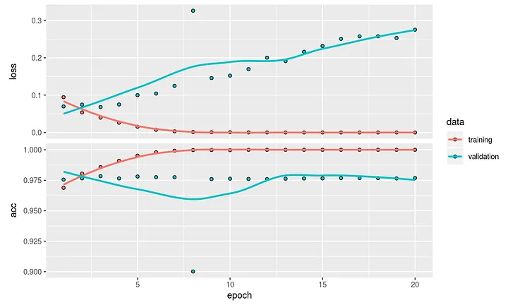
The plot might show us why it is so important to use a train and test set to avoid overfitting. After about 10 epochs the performance in the validation set is stabilizing and no improvement is recorded in the validation set. We extract the weights of the model to look at our 32 embedding dimensions. Below you will see the dimension for word number 495 / aanraden.
# get embedding matrix, the weights from the model
word2vec_embedding <- get_weights(model)[[1]]

# give the index back the name of the word for looking up a word embedding (NA for blanks)
rownames(word2vec_embedding) <- c('NA',as.vector(unlist(tokenizer_train$index_word)))

# let's look up word 495 ("aanraden") again, the index shifted with 1 as NAs are now on top of the list
print(rownames(word2vec_embedding)[496])
word2vec_embedding[495,]
[1] "aanraden"
 [1]  0.135066003  0.099465132  0.292932719  0.339372128  0.167709514
 [6] -0.064011954 -0.212190494  0.247801170 -0.138503119 -0.178294301
[11] -0.178855255 -0.212001726  0.067998052  0.041063324 -0.045047209
[16] -0.043304760 -0.166447461  0.161533043  0.156035781 -0.112948038
[21]  0.185008273 -0.212475866  0.191676199 -0.315667540 -0.146218479
[26]  0.081838161  0.003491634  0.173275918 -0.181478009 -0.017451271
[31] -0.200740322 -0.125586092
As every word has these 32 dimensions we can now calculate the L2 distance between words and find out which words are close to pasta and bier (‘beer’). As you can see pizza is very close to pasta but also groente (‘vegetable’), kaas (‘cheese’) and warm. That pasta and pizza are similar words is no surprise. But apparently reviewers also mention a pasta with rijst ( ‘rice’) involved.
As for the word bier (‘beer’) we see words like huiswijn (‘housewine’), fruit but also words as vraag (‘question’) and tafeltjes (‘tables’). Yes, these are words you might expect to be similar. Yet, I’m not blown away by these results. In the next section we will use an alternative and build a GloVe embedding model to see how that works out.
# find words that are related to another word
token <- "pasta"
embedding_vector <- t(matrix(word2vec_embedding[token,]))
cos_sim = sim2(x = word2vec_embedding, y = embedding_vector, method = "cosine", norm = "l2")
cat(paste0('Words from the embedding layer similar to "pasta":', '\n'))
print(head(sort(cos_sim[,1], decreasing = TRUE), 10))

token <- "bier"
embedding_vector <- t(matrix(word2vec_embedding[token,]))
cos_sim = sim2(x = word2vec_embedding, y = embedding_vector, method = "cosine", norm = "l2")
cat(paste0('\n', 'Words from the embedding layer similar to "bier":', '\n'))
print(head(sort(cos_sim[,1], decreasing = TRUE), 10))
Words from the embedding layer similar to "pasta":
pasta, pizza, groente, kaas, verwacht, klaargemaakt, zat, warm, rijst, persoon

Words from the embedding layer similar to "bier":
bier, decor, huiswijn, fruit, staat, wilt, tafeltjes, vraag, krijg    aardig
Training a GloVe word embedding
So at face value the results from Word2Vec were not mind-blowing. Some say that Word2Vec’s training performs better when using larger vocabularies and hyper parameter tuning needs to be done to achieve the best results. There is an alternative on the block: Global Vectors for Word Representation. Like Word2vec, GloVe uses vector representations for words and the distance between words is related to semantic similarity. However, GloVe focuses on words co-occurrences over the entire corpus. Its embeddings relate to the probabilities that two words appear together. This is the case because GloVe is a count-based model where dimensionality reduction is done on the co-occurrence of words that appear together. Word2Vec is using a probabilistic approach where a target word and context words are predicted (and optimized based on the loss function). Many favor a GloVe model over a classic Word2Vec model because of the fact that global information is better captured, it simply works better for many tasks. So let’s find out how a GloVe model is working out for our restaurant reviews.
We re-use our reviews_new dataset, which is already cleaned, as input for text2vec. As you can see terms like restaurant and eten (‘food’) are most common and time indications and numbers are rare.
library(text2vec)

# We need to tokenize our already tokenized set as input for text2vec, re-use cleaned text in reviews_new
it <- itoken(reviews_new$reviewTextClean,
                   tokenizer = word_tokenizer,
                   ids = reviews_new$restoReviewId,
                   progressbar = TRUE)

# create a vocabulary out of the tokenset (stopword removal and bi-grams are optional)
vocab <- create_vocabulary(it) # use uni-grams

# text2vec has the option to prune the vocabulary of low-frequent words
vocab <- prune_vocabulary(vocab, term_count_min = 5)

# What's in the vocabulary?
print(vocab)
Number of docs: 145867
0 stopwords:  ...
ngram_min = 1; ngram_max = 1
Vocabulary:
             term term_count doc_count
    1:       0000          5         5
    2:         02          5         4
    3:       0300          5         5
    4:         06          5         5
    5:        104          5         5
   ---
37516: restaurant      64841     47930
37517:     lekker      68548     50218
37518:  bediening      78009     68484
37519:       goed      88603     61218
37520:       eten     111636     75699
Next we vectorize our input tokens and create a Term-Count-Matrix for GloVe to handle. We create a matrix for the word embeddings (glove_model) and execute the glove command from the text2vec package that will create the embedding matrix with (again) 32 dimension. The GloVemodel learns two sets of word vectors: main and context. Best practice is to combine both the main word vectors and the context word vectors into one matrix.
# Vectorize word to integers
vectorizer <- vocab_vectorizer(vocab)

# Create a Term-Count-Matrix, by default it will use a skipgram window of 5 (symmetrical)
tcm <- create_tcm(it, vectorizer, skip_grams_window = 5L)

# maximum number of co-occurrences to use in the weighting function, we choose the entire token set divided by 100
x_max <- length(vocab$doc_count)/100

# set up the embedding matrix and fit model
glove_model <- GloVe$new(rank = 32, x_max = x_max)
glove_embedding = glove_model$fit_transform(tcm, n_iter = 20, convergence_tol = 0.01, n_threads = 4)

# combine main embedding and context embeddings (sum) into one matrix
glove_embedding = glove_embedding + t(glove_model$components) # the transpose of the context matrix
Let’s find out how well GloVe is doing on our restaurant reviews. We pull up the same nearby words as we did earlier. These results look much better, a translation to English is not even required, everybody can see that pasta, spaghetti, lasagne, pizza and risotto are semantically very close. This also holds for bier (‘beer’): tap, biertjes (‘beers’), glas and alcoholvrij (‘without alcohol’) . So based on this small comparison the GloVe word embedding does a far better job than a classic Words2Vec model on our corpus. However, these results are at this point no indication that GloVe will perform better in downstream predictions tasks. To show you results of our efforts in more detail side by side we will visualize the embeddings in the next section.
word <- glove_embedding["pasta", , drop = FALSE] # wat ligt er dicht bij 'lekker'
cos_sim = sim2(x = glove_embedding, y = word, method = "cosine", norm = "l2")
head(sort(cos_sim[,1], decreasing = TRUE), 10)

word <- glove_embedding["bier", , drop = FALSE]
cos_sim = sim2(x = glove_embedding, y = word, method = "cosine", norm = "l2")
head(sort(cos_sim[,1], decreasing = TRUE), 10)
pasta, pizza, lasagne, spaghetti, risotto, ravioli, zeevruchten, vongole, paddenstoelen, pizzasbier, tap, biertje, biertjes, fles, glas, flesje, wijn, frisdrank, alcoholvrij
Visualization
Up till now we’ve been looking at code, matrices en characters to see how both techniques are doing. In this section we will visualize the results of both techniques. Viewing 32 dimensions is impossible, so we need some form of data reduction. We need a method that is both fast en suitable for high dimensionality reduction. UMAP is the technique we are going to be using here, mainly because it is fast and has the ability to balance between local and global proximity very well. Another candidate for dimension reduction would be t-SNE, an excellent blog on the differences between t-SNE and UMAP can be found here.
UMAP has a lot of parameters you can play around with, the most important are n_neighbors and min_dist. As you might have read in the above blog a first thing that UMAP does is to create a high dimensional map, and the number of neighbors connected to a single point determine what that map looks like. The initial state of the map will have a focus on local detailed connections with a low value for n_neighbors and a more global big picture with a higher value of n_neighbors. Second the min_dist parameter will determine how many space you allow between points. A low value will result in close clusters at a local level, a high value will yield a more loosely connected picture.
We reduce our number of embedding dimensions (32) to just 2 so we can visualize results easily using an X and Y plot. Using 3 dimensions would also be nice, but ggplot does not allow for a 3D render in this notebook.
# Word2Vec dimension reduction
word2vec_umap <- umap(word2vec_embedding, n_components = 2, metric = "cosine", n_neighbors = 25, min_dist = 0.1, spread=2)

# GloVe dimension reduction
glove_umap <- umap(glove_embedding, n_components = 2, metric = "cosine", n_neighbors = 25, min_dist = 0.1, spread=2)

# Dimensions of end result
dim(glove_umap)
[1] 37520 2
We did a few iterations to find out which UMAP parameter settings gave the best results. Now for both Word2Vec and GloVe embeddings we have reduced the number of dimensions to 2. Below we attach the words that belong to rows and we create a dataframe as input for ggplot.
# Put results in a dataframe for ggplot, starting with Word2Vec
df_word2vec_umap <- as.data.frame(word2vec_umap, stringsAsFactors = FALSE)

# Add the labels of the words to the dataframe
df_word2vec_umap$word <- rownames(word2vec_embedding)
colnames(df_word2vec_umap) <- c("UMAP1", "UMAP2", "word")
df_word2vec_umap$technique <- 'Word2Vec'
cat(paste0('Our Word2Vec embedding reduced to 2 dimensions:', '\n'))
str(df_word2vec_umap)

# Do the same for the GloVe embeddings
df_glove_umap <- as.data.frame(glove_umap, stringsAsFactors = FALSE)

# Add the labels of the words to the dataframe
df_glove_umap$word <- rownames(glove_embedding)
colnames(df_glove_umap) <- c("UMAP1", "UMAP2", "word")
df_glove_umap$technique <- 'GloVe'
cat(paste0('\n', 'Our GloVe embedding reduced to 2 dimensions:', '\n'))
str(df_glove_umap)

# Combine the datasets
df_umap <- bind_rows(df_word2vec_umap, df_glove_umap)
Our Word2Vec embedding reduced to 2 dimensions:
'data.frame':	37488 obs. of  4 variables:
 $ UMAP1    : num  7.45 8.1 8.35 8.16 8.34 ...
 $ UMAP2    : num  1.233 -0.677 -0.06 -0.563 0.136 ...
 $ word     : chr  "NA" "eten" "goed" "bediening" ...
 $ technique: chr  "Word2Vec" "Word2Vec" "Word2Vec" "Word2Vec" ...

Our GloVe embedding reduced to 2 dimensions:
'data.frame':	37520 obs. of  4 variables:
 $ UMAP1    : num  -3.186 -5.385 -1.964 -0.682 1.685 ...
 $ UMAP2    : num  0.252 1.316 -1.336 1.24 0.333 ...
 $ word     : chr  "0000" "02" "0300" "06" ...
 $ technique: chr  "GloVe" "GloVe" "GloVe" "GloVe" ...
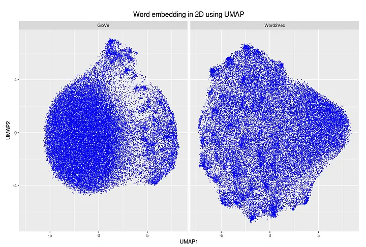
On the left we see the dimension reduction for the GloVe model and on the right the Word2Vec image. There are clearly more distinct spaces between local clusters for the GloVe model, the Word2Vec model looks more dense.
# Plot the UMAP dimensions for both Word2Vec and GloVe
ggplot(df_umap) +
      geom_point(aes(x = UMAP1, y = UMAP2), colour = 'blue', size = 0.05) +
      facet_wrap(~technique) +
      labs(title = "Word embedding in 2D using UMAP") +
      theme(plot.title = element_text(hjust = .5, size = 14))
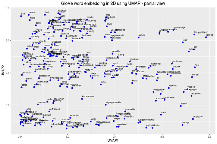
Let’s zoom in on the GloVe embedding some more an plot labels for all the embedding points. On the bottom left we clearly have a spot for desert related words (brownies, citroentaart ‘lemon cake’, spekkoek ‘layer cake’). On the top right we have things that went wrong (teruggestuurd ‘sent back’, lauw ‘lukewarm’, bevroren ‘frozen’) and on the middle left we have a spot for snacks (bitterballen ‘bitterballs’, mayonaise, kipnuggets, frikandellen ‘meat balls’). These embeddings clearly show that with this technique we are able to cluster words together that have the same semantic meaning.
# Plot the bottom part of the GloVe word embedding with labels
ggplot(df_glove_umap[df_glove_umap$UMAP1 > 3.0 & df_glove_umap$UMAP1 < 3.8 & df_glove_umap$UMAP2 > 4.6,]) +
      geom_point(aes(x = UMAP1, y = UMAP2), colour = 'blue', size = 2) +
      geom_text(aes(UMAP1, UMAP2, label = word), size = 2.5, vjust=-1, hjust=0) +
      labs(title = "GloVe word embedding in 2D using UMAP - partial view") +
      theme(plot.title = element_text(hjust = .5, size = 14))
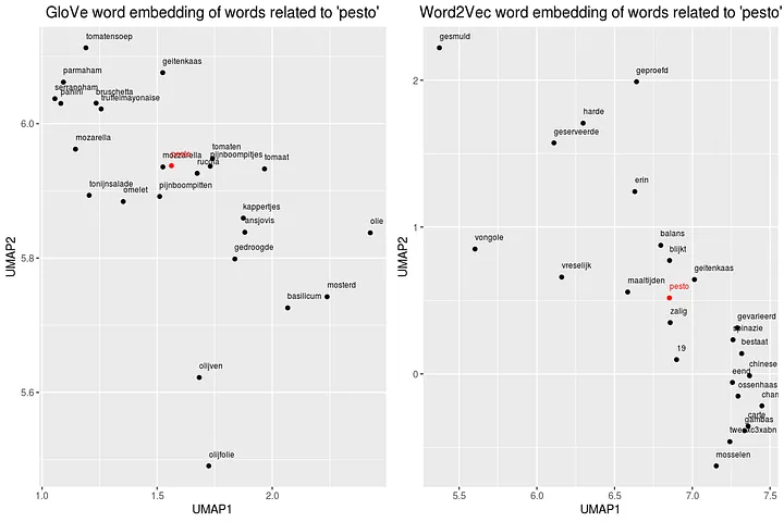
We can also take a single word from the index for both techniques and plot semantically close words to see differences between GloVe and Word2Vec. We choose for the word pesto as it has many ingredients, can be used in various dishes and not everybody likes the taste. First we gather words that are close (based on the L2 distance), save results in a dataframe and plot results. These plots are crystal clear, the GloVe model does a far better job in understand relationship between words in our restaurant reviews.
# Plot the word embedding of words that are related for the GloVe model
word <- glove_embedding["pesto", , drop = FALSE]
cos_sim = sim2(x = glove_embedding, y = word, method = "cosine", norm = "l2")
select <- data.frame(rownames(as.data.frame(head(sort(cos_sim[,1], decreasing = TRUE), 25))))
colnames(select) <- "word"
selected_words <- df_glove_umap %>% inner_join(y=select, by= "word", match = "all")

#The ggplot visual for Word2Vec
pesto_glove <- ggplot(selected_words, aes(x = UMAP1, y = UMAP2, colour = word == 'pesto')) +
      geom_point(show.legend = FALSE) +
      scale_color_manual(values = c('black', 'red')) +
      geom_text(aes(UMAP1, UMAP2, label = word), show.legend = FALSE, size = 2.5, vjust=-1.5, hjust=0) +
      labs(title = "GloVe word embedding of words related to 'pesto'") +
      theme(plot.title = element_text(hjust = .5, size = 14))

# And so the same for the Word2Vec model
token <- "pesto"
embedding_vector <- t(matrix(word2vec_embedding[token,]))
cos_sim = sim2(x = word2vec_embedding, y = embedding_vector, method = "cosine", norm = "l2")
select <- data.frame(rownames(as.data.frame(head(sort(cos_sim[,1], decreasing = TRUE), 25))))
colnames(select) <- "word"
selected_words <- df_word2vec_umap %>% inner_join(y=select, by= "word", match = "all")

# The ggplot visual for GloVe
pesto_word2vec <- ggplot(selected_words, aes(x = UMAP1, y = UMAP2, colour = word == 'pesto')) +
      geom_point(show.legend = FALSE) +
      scale_color_manual(values = c('black', 'red')) +
      geom_text(aes(UMAP1, UMAP2, label = word), show.legend = FALSE, size = 2.5, vjust=-1.5, hjust=0) +
      labs(title = "Word2Vec word embedding of words related to 'pesto'") +
      theme(plot.title = element_text(hjust = .5, size = 14))

library(gridExtra)

# Put the results side-by-side for a comparison
grid.arrange(pesto_glove,pesto_word2vec, ncol=2)
Word embedding — wrapping it up
In this article we have explained what word embedding is and showed you how you can train your own embedding model using two different techniques. We used real world data of restaurant reviews which turned out very well for the GloVe model and not so well for the Word2Vec model. Building these embedding models required quite some decision making in order to find ‘the best’ model. Of course you can always avoid making all these decisions and use a pre-trained model as input for your analyses. More on the usage of pre-trained embedding models in an upcoming article.
Now that we have a well trained GloVe word embedding model, how are we going to leverage the knowledge we gained? In a next article we will compare performances for predicting which restaurant is likely to receive a next Michelin star using NLP techniques. Next to the reviewers text left behind after a restaurant visit we also have some other features about the review to predict whether the review is a Michelin review or not. We will combine the knowledge gained from the word embedding and enrich the dataset with these additional features for our predictions.
This article is of part of our NLP with R series. An overview of all articles within the series can be found here.
- Previous in this series: Topic Modeling
- Next up in this series: Predicting using Topic Model results
Do you want to do this yourself? Please feel free to download the Databricks Notebook or the R-script from out gitlab page.
