Identify topics in restaurant reviews
In a sequence of articles we compare different NLP techniques to show you how we get valuable information from unstructured text. About a year ago we gathered reviews on Dutch restaurants. We were wondering whether ‘the wisdom of the crowd’ — reviews from restaurant visitors — could be used to predict which restaurants are most likely to receive a new Michelin-star. Read this post to see how that worked out. We used topic modeling as our primary tool to extract information from the review texts and combined that with predictive modeling techniques to end up with our predictions.
We got a lot of attention with our predictions and also questions about how we did the text analysis part. To answer these questions, we will explain our approach in more detail in the coming articles. But we didn’t stop exploring NLP techniques after our publication, and we also like to share insights from adding more novel NLP techniques. More specifically we will use two types of word embeddings — a classic Word2Vec model and a GLoVe embedding model — we’ll use transfer learning with pretrained word embeddings and we use BERT. We compare the added value of these advanced NLP techniques to our baseline topic model on the same dataset. By showing what we did and how we did it, we hope to guide others that are keen to use textual data for their own data science endeavors.
In a previous article we showed how we prepared our data to be used for various NLP techniques. Here, we commence our series of articles on NLP techniques by introducing Topic Modeling and show you how to identify topics, visualize topic model results. In a later article, we show you how to use the topic model results in a predictive model.
What is Topic Modeling?
To discover the topics that restaurant reviewers write about in their restaurant reviews, we use Topic Modeling. But what is a Topic Model? In machine learning and natural language processing, a topic model is a type of statistical model that can be used for discovering the abstract topics that occur in a collection of documents. There are a number of algorithms to extract topics from a collection of texts, but the Latent Dirichlet Allocation is one of the most popular algorithms because it is efficient en results in highly interpretable topics. Interpretability of topics is an important feature of a topic model, since we do not only want to find statistically relevant groupings of words, we also want to be able to label the identified topics with a topic name that others can relate to. As such, topic modeling has some similarities to clustering techniques like KMeans, where interpretation is also as important as statistical metrics are in determining what is a ‘good’ solution. How topic modeling / LDA works, is visualized by Blei as:
As the figure shows:
- Each topic is a distribution over words
- Each document is a distribution over topics
So after we are done topic modeling our reviews:
- we should know what are topics or subjects that reviewers write about in their restaurant reviews,
- we know what tokens or words are most important in these topics, and
- we can tell for each individual review to what extent it is about the identified topics and this can be a mix — 80% about topic X and 20% about topic Y.
Step 0: Setting up our context
First, we set up our workbook environment with the required packages to perform topic modeling.
In our blog on preparing the textual data we already briefly introduced tidyverse and tidytext. Here, we add a few other packages to the list:
- topicmodels is a package to estimate topic models with LDA and builds upon data structures created with the tm package
- tm is a powerful, generic package with all sorts of text mining functionality, among which creating document term matrices, which we need for topic modeling
- ldavis is a great package to visualize and interpret the topic model and a very helpful when labeling topics
# Loading packages
library(tidyverse)
library(tidytext)
library(topicmodels)
library(tm)
library(LDAvis)
Step 1. Load preprocessed data
Before we delve into the analytical side of things, we need some prepared textual data. As all true data scientists know, proper data preparation takes most of your time and is most decisive for the quality of the analysis results you end up with. Preparing textual data is another cup of tea compared to preparing structured numeric or categorical data. In this blog our focus is on text analytics. Yet we do want to show you how we cleaned and prepared the data we gathered. In this previous blog, we explain in detail how we preprocessed the data, resulting in the following 5 files we can use in our NLP analytics:
- reviews.csv: a csv file with original and prepared review texts — the fuel for our NLP analyses. (included key: restoreviewid, hence the unique identifier for a review)
- labels.csv: a csv file with 1 / 0 values, indicating whether the review is a review for a Michelin restaurant or not (included key: restoreviewid)
- restoid.csv: a csv file with restaurant id’s, to be able to determine which reviews belong to which restaurant (included key: restoreviewid)
- trainids.csv: a csv file with 1 / 0 values, indicating whether the review should be used for training or testing — we already split the reviews in train/test to enable reuse of the same samples for fair comparisons between techniques (included key: restoreviewid)
- features.csv: a csv file with other features regarding the reviews (included key: restoreviewid)
These files with the cleaned and relevant data for NLP techniques are made available to you via public blob storage so that you can run all code we present yourself and see how things work in more detail. For our topic model, we need three of these files:
# **reviews.csv**: a csv file with review texts - the fuel for our NLP analyses.
#  (included key: restoreviewid, hence the unique identifier for a review)
reviews <- read.csv(
  file = 'https://bhciaaablob.blob.core.windows.net/cmotionsnlpblogs/reviews.csv',
  header=TRUE,stringsAsFactors=FALSE)

# **labels.csv**: a csv file with 1 / 0 values, indicating whether the review is a review for
# a Michelin restaurant or not  (included key: restoreviewid)
labels <- read.csv(
  file = 'https://bhciaaablob.blob.core.windows.net/cmotionsnlpblogs/labels.csv',
  header=TRUE,stringsAsFactors=FALSE)

# **trainids.csv**: a csv file with 1 / 0 values, indicating whether the review should be used
# for training or testing - we already split the reviews in train/test to enable reuse of the
# same samples for fair comparisons between techniques (included key: restoreviewid)
set.seed(1234)
trainids <-   read.csv(
  file = 'https://bhciaaablob.blob.core.windows.net/cmotionsnlpblogs/trainids.csv',
  header=TRUE,stringsAsFactors=FALSE) %>% mutate(rv = runif(nrow(.)))
Step 2: Prepare data for topic modeling
Starting from the cleaned review texts, we have to do some things before we can estimate our topic models:
- Tokenize our prepared text (including bigrams)
- Sample reviews for training our topic model
- Filter relevant tokens
- Create Document Term Matrix
2.1. Tokenize our prepared text (including bigrams)
Latent Dirichlet Allocation (LDA), the technique we use for topic modeling, is a ‘bag of words’ technique. What this means, is that the NLP technique does not look at the order of the tokens when analyzing the text. Hence, where the token is located in the text and what other tokens are close to the token (preceding / subsequent tokens) within the document is not considered. It’s like all tokens from the document text are thrown into a bag, mixing them up but retaining the information that the tokens are in the same document. As a result, we might miss out on crucial information if a lot of interesting collocations — frequent combinations of tokens — are present in the text. Popular examples are names of people (‘Donald Trump’, ’Jonnie Boer’) or places (‘United States’, ‘Den Haag’) but also context-specific combinations of words might be important to include in our topic model: ‘witte wijn’ (‘white wine’), ‘rode wijn’, (‘red wine’), ‘gaan eten’ (‘go eat’). To make sure we don’t miss out on these important collocations, we add the prepared bigrams that are present in our text. Remember that we already removed stopwords and interpunction in our dataprep.
After adding bigrams to the loaded, cleaned texts, we split the texts again to end up with a dataframe where each row is a review — token combination. We filter out reviews that have become too short (<25 tokens) after removing stop words. In this format, we’re ready for our last preparations before we can start modeling topics.
## combine unigrams and bigrams into reviewTextClean and divide text into separate words
reviews_tokens <- reviews %>%
    mutate(reviewTextClean = paste0(reviewTextClean,bigrams)) %>%
    select(restoReviewId, reviewTextClean) %>%
    unnest_tokens(token, reviewTextClean) %>%
    # filter out reviews with less than 25 tokens
    group_by(restoReviewId) %>% mutate(n_tokens = n()) %>% filter(n_tokens>=25) %>%
    ungroup() %>% select(-n_tokens)

# summarize result after tokenization
str(reviews_tokens)

#tibble [8,681,554 × 2] (S3: tbl_df/tbl/data.frame)
# $ restoReviewId: chr [1:8681554] "255757_1" "255757_1" "255757_1" "255757_1" ...
# $ token        : chr [1:8681554] "heerlijk" "eten" "leuke" "sfeer" ...
2.2 Sample reviews for training our topic model
In our next step, we will filter the most relevant tokens to include in the document term matrix and subsequently in topic modeling. But first we need to determine which documents (reviews) are most important to us. For some reasons we do not want to use all reviews as input for our topic model:
- In the end, we want to use the topics in a prediction model to predict Michelin stars. It’s best practice to set aside a test set before we build the topic model and use its outcomes in the downstream predictive task. This way we build both our topic model and our prediction on train data and keep test data unseen until evaluation.
- As shown below, no more than 3% of all reviews are Michelin reviews. By increasing the proportion of Michelin reviews in the train set we use for topic modeling, it is more likely that specific topics that are discussed in Michelin reviews will be identified.
For these reasons, we will focus the rest of the preparation towards our topic model and estimation of the topic models on a subset of reviews. This subset contains only reviews that are already specified as training cases in our data preparation notebook. Within this subset, we take all Michelin reviews (about 3.000) and complement with non-Michelin reviews to end up with around 10.000 reviews:
# what % of all reviews are Michelin reviews?
labels %>% group_by(ind_michelin) %>% summarize(n=n()) %>% mutate(pct=scales::percent(n/sum(n)))
# A tibble: 2 x 3
  ind_michelin      n pct
         <int>  <int> <chr>
1            0 141554 97%
2            1   4313 3%
# sample reviews: Take all michelin train reviews and complement with
# non-michelin train cases to include 10K reviews in total
reviews_tokens_train <- reviews_tokens %>%
    inner_join(labels,by = "restoReviewId") %>%
    inner_join(trainids,by = "restoReviewId") %>%
    mutate(train_smpl = case_when(
             # sample all reviews that are michelin review and in the train subset
             train==1 & ind_michelin == 1 ~ 1,
             # complete 10K sample by adding 7.1K reviews from non-michelin train reviews
             train==1 & rv < (7100/95000) ~ 1,
             # all other reviews are not in the train_smpl
             TRUE~0))

# what reviews will we keep?
reviews_tokens_train %>% group_by(train_smpl,train,ind_michelin) %>%
  summarize(n_reviews=n_distinct(restoReviewId),n_tokens=n_distinct(token)) %>% print()

#create train data using train_smpl as filter
reviews_tokens_train <- reviews_tokens_train %>% filter(train_smpl == 1)

sprintf('%s unique reviews and %s unique tokens selected to train topic model',
    n_distinct(reviews_tokens_train$restoReviewId),n_distinct(reviews_tokens_train$token))
# A tibble: 5 x 5
# Groups:   train_smpl, train [3]
  train_smpl train ind_michelin n_reviews n_tokens
       <dbl> <int>        <int>     <int>    <int>
1          0     0            0     40997   433179
2          0     0            1      1290    35129
3          0     1            0     88505   773887
4          1     1            0      7181   111435
5          1     1            1      2971    70548
[1] "10152 unique reviews and 163137 unique tokens selected to train topic model"
2.3 Filter tokens
Now that we’ve added bigrams to the tokens and we’ve re-tokenized our texts, we still have many, many unique tokens available for our topic model. It’s best practice to get rid of the longtail of infrequent terms. Let’s first have a look at what the distribution of token frequency looks like. Remember that in our data preparation blog we already removed all stop words from the texts, including 128 custom high frequency ‘stop’ words that we specified by looking at the token frequency in preparing the data.
reviews_tokens_train %>%
  group_by(token) %>% summarize(token_freq=n()) %>%
  mutate(token_freq_binned = case_when(token_freq>20~20,TRUE~as.numeric(token_freq))) %>%
  group_by(token_freq_binned) %>% summarise(n_tokens = n()) %>%
  mutate(pct_tokens = n_tokens/sum(n_tokens),
         cumpct_tokens = cumsum(n_tokens)/sum(n_tokens)) %>%
  ggplot(aes(x=token_freq_binned)) +
          scale_y_continuous(labels = scales::percent_format(accuracy = 1)) +
          geom_bar(aes(y=pct_tokens),stat='identity',fill='blue') +
          geom_line(aes(y=cumpct_tokens),stat='identity',color='orange',linetype='dashed') +
          geom_text(aes(y=cumpct_tokens,label=scales::percent(cumpct_tokens,accuracy=1)),
                    size=3) + theme_minimal() +
          ggtitle("Frequency of token in Corpus (all reviews)") + xlab("token frequency") +
          ylab("% of all tokens")
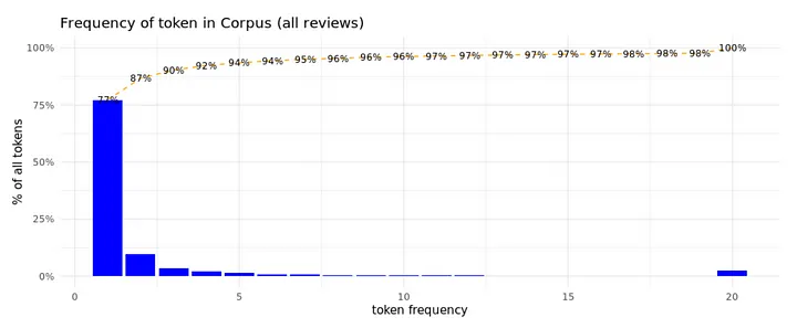
The plot above clearly shows that a huge amount of the unique tokens occurs rarely in all the reviews, 75% occurs only once.
Focus on tokens that occur 5 times or more in train Corpus
As we can see from the token frequency count, there are a lot of tokens that occur only once or a few times: Around 92% of all unique tokens occur less than 5 times in our corpus of reviews. These low frequency tokens impact the topic model analysis. To focus on frequently used tokens, we select tokens that occur 5 times or more in the prepared train data. This is hopefully enough to learn topics from tokens that occur together in the same reviews. In optimizing our topic model, we can vary the minimum frequency to evaluate impact on results.
Why not TF-IDF?
Having read some on text analytics tools, you might wonder: Why don’t we use TF-IDF to select most relevant tokens? TF-IDF stands for Term Frequency — Inverse Document Frequency. This metric combines the Term Frequency — how often is the token present in a document? — with the Inverse of the Document Frequency — in how many unique documents is the term present? Although the TF-IDF is often a good choice to select most relevant tokens, it is not in our context, where the document size is limited and reoccurrence of the same token in the same text is low. Not often, a token has a Term Frequency above 1. As a result, only the Inverse Document Frequency part is decisive and this favors the tokens that only occur in one or two reviews. For this reason, we do not use TF-IDF here, but look at overall frequency to pick relevant tokens for topic modeling. Also because we already removed the custom list of stop words from our text, hence too frequent tokens are already removed.
By filtering the infrequent tokens, we’ve decreased the number of tokens to consider in our LDA dramatically, focusing on the 12K (8%) most frequent tokens and removing the 146K (92%) tokens that are too infrequent in the corpus. These selected tokens do still represent 73% of all the tokens in the documents though:
reviews_tokens_train %>%
  group_by(token) %>% summarize(token_freq=n()) %>%
  mutate(min_5_freq = case_when(token_freq<5~'token frequency: <5',
                                TRUE~'token frequency: >=5')) %>%
  group_by(min_5_freq) %>% summarise(n_unique_tokens = n(),n_tokens=sum(token_freq)) %>%
  mutate(pct_unique_tokens = scales::percent(n_unique_tokens / sum(n_unique_tokens)),
         pct_all_tokens=scales::percent(n_tokens / sum(n_tokens)))
# A tibble: 2 x 5
min_5_freq n_unique_tokens n_tokens pct_unique_tokens pct_all_tokens
  <chr>                          <int>    <int> <chr> <chr>
1 token frequency: <5           150612   187523 92%   27%
2 token frequency: >=5           12525   518146 8%    73%
2.4 Create DTM
After filtering the tokens we want to use to build our topic model, we can create the input for LDA. This requires a document-term-matrix or DTM hence a matrix with in the rows all our documents (reviews) and in the columns all the terms (the relevant tokens). Do note that we use the overall token frequency for the value parameter. You might expect the document specific term frequency here, however we use the overall token frequency to give much more emphasis in finding the topic model to terms that are more frequent in general; given the short length of reviews (compared to books or articles that are often used in topic modeling) the probability of a single token to occur more often in the review is limited.
# remove infrequent tokens
reviews_tokens_train_smpl <- reviews_tokens_train %>%
  group_by(token) %>% mutate(token_freq=n()) %>%  filter(token_freq>=5)

# create document term matrix
dtm <- reviews_tokens_train_smpl %>%
  cast_dtm(document = restoReviewId,term = token,value = token_freq)

#check dimenstions of dtm
cat(paste0('DTM dimensions: Documents (',dim(dtm)[1],') x Tokens (',dim(dtm)[2],')',
           ' (average token frequency: ',round(sum(dtm)/sum(dtm!=0),2),')'))
DTM dimensions:
Documents (10152) x Tokens (12525) (average token frequency: 702.3)
Step 3: Develop Topic model
Now that we have a DTM, we’re ready to start topic modeling! So far, we already made quite some choices with impact on our analysis result: what minimal review length to use, what stop words to exclude, what n-grams to include, the minimal token frequency to use tokens… And a few more choices need to be made.
LDA has a number of parameters that impact the outcome, of which the most important are:
- k: The number of topics! Yes, this is a parameter and not an outcome. Similar to clustering techniques like Kmeans, you need to tell how many clusters/topics you want to identify.
- method: The topicmodels package enables different optimization methods, VEM algorithm or Gibbs sampling, default is VEM.
- control: list of control variables to guide estimation — relevant parameters depend on chosen method VEM or Gibbs but most important ones are:
- nstart: The number of runs to perform with the same settings but different seeds
- seed: For reproducibility a random seed can be set. If nstart > 1, you need to provide multiple seeds, 1 per nstart (eg. c(‘123’,’234′,’345′))
- best: If TRUE (default), only the run with the best fitting result is kept, of set, if FALSE a list of all runs is returned so you can examine all of them.
For a full overview of all parameters and settings available, see the topicmodels package vignette.
Estimate LDA Topic Model
Most impactful parameter is k: the number of topics to identify. How to pick a value for k? This is partly a result of discussion (what number of topics do we expect to find in this context?) and trial & error (try different values of k, evaluate results). Some data scientists might not like this, they prefer to look at statistics to guide them in this process, but for those familiar with other unsupervised data science techniques like Kmeans this is not that new. Clustering and also topic modeling is to some extent more art than science. Guided by statistical techniques and measures, a data scientist sculpts a topic modeling solution that fits the (business) needs. In case you do need a starting point for k with some statistical background, you can try this approach or this approach.
Let’s start with a topic model to identify 3 topics and explore the result. We have no reason to change any other defaults at this point.
lda_fit <- LDA(dtm, k = 3)
Evaluate Topic Model
Topic model is fitted, so, let’s explore!
The fitted lda object contains a number of matrices:
- phi: matrix with distribution of tokens (in rows) over topics (in columns)
- theta: matrix with distribution of documents (hence: reviews, in rows) over topics (in columns)
Both for phi and for theta, the sum over all columns is equal to 1, meaning:
- For phi, the sum of all token scores within a topic is 1 — higher scores meaning higher importance of that token within the topic.
- For theta, the sum of all topic scores within a document is 1 — higher scores meaning the topic is more present in that document.
# phi (topic - token distribution matrix) -  topics in rows, tokens in columns:
phi <- posterior(lda_fit)$terms %>% as.matrix
cat(paste0('Dimensions of phi (topic-token-matrix): ',paste(dim(phi),collapse=' x '),'\n'))
cat(paste0('phi examples (8 tokens): ','\n'))
phi[,1:8] %>% as_tibble() %>% mutate_if(is.numeric, round, 5) %>% print()

# theta (document - topic distribution matrix) -  documents in rows, topic probs in columns:
theta <- posterior(lda_fit)$topics %>% as.matrix
cat(paste0('\n\n','Dimensions of theta (document-topic-matrix): ',
           paste(dim(theta),collapse=' x '),'\n'))

cat(paste0('theta examples (8 documents): ','\n'))
theta[1:8,] %>% as_tibble() %>% mutate_if(is.numeric, round, 5) %>%
  setNames(paste0('Topic', names(.))) %>% print()
Dimensions of phi (topic-token-matrix): 3 x 12525
phi examples (8 tokens):
# A tibble: 3 x 8
  zeldzaam slechte   avond service  niveau    eten    goed vanavond
     <dbl>   <dbl>   <dbl>   <dbl>   <dbl>   <dbl>   <dbl>    <dbl>
1        0 0.00006 0.00295 0.00001 0.00021 0.00022 0.112   0.0001
2        0 0.00041 0.00936 0.00843 0.00032 0.430   0.00277 0.0001
3        0 0.00002 0.0157  0.00412 0.00086 0.00003 0.112   0.000070


Dimensions of theta (document-topic-matrix): 10152 x 3
theta examples (8 documents):
# A tibble: 8 x 3
   Topic1  Topic2 Topic3
    <dbl>   <dbl>  <dbl>
1 0       0.603    0.397
2 0       0.319    0.681
3 0       0.445    0.555
4 0.00001 0.00001  1.00
5 0.340   0        0.660
6 0       0.424    0.576
7 0.00001 0.00001  1.00
8 0.220   0.467    0.313
To explore our topic model, let’s start by looking at the most important tokens per topic. To do so, we need to specify when a token is important for a topic. We could argue that the token is important for the topic when it has a high probability to occur within a topic p(token|topic). Let’s see how this looks for our 3-topics topic model. We’ll use a neat function of the tidytext package, that helps preparing the topic model data to visualize most important tokens per topic: tidy().
# get token probability per token per topic
topics <- tidy(lda_fit)

# only select top-10 terms per topic based on token probability within a topic
plotinput <- topics %>%
  mutate(topic = as.factor(paste0('Topic',topic))) %>%
  group_by(topic) %>%
  top_n(10, beta) %>%
  ungroup() %>%
  arrange(topic, -beta)

# plot highest probability terms per topic
names <- levels(unique(plotinput$topic))
colors <- RColorBrewer::brewer.pal(n=length(names),name="Set2")

plist <- list()

for (i in 1:length(names)) {
  d <- subset(plotinput,topic == names[i])[1:10,]
  d$term <- factor(d$term, levels=d[order(d$beta),]$term)

  p1 <- ggplot(d, aes(x = term, y = beta, width=0.75)) +
  labs(y = NULL, x = NULL, fill = NULL) +
  geom_bar(stat = "identity",fill=colors[i]) +
  facet_wrap(~topic) +
  coord_flip() +
  guides(fill=FALSE) +
  theme_bw() + theme(strip.background  = element_blank(),
                     panel.grid.major = element_line(colour = "grey80"),
                     panel.border = element_blank(),
                     axis.ticks = element_line(size = 0),
                     panel.grid.minor.y = element_blank(),
                     panel.grid.major.y = element_blank() ) +
  theme(legend.position="bottom")

  plist[[names[i]]] = p1
}

library(gridExtra)
do.call("grid.arrange", c(plist, ncol=3))
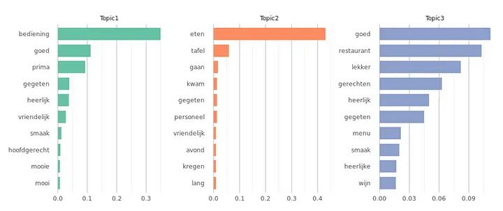
With this plot, we get a first feel of what the topics in our first topic model represent. As we can see from the plot, looking at the token probability per topic has the downside that tokens that have a high overall frequency have a higher probability to show up in the top-10 for multiple topics. For instance restaurant shows up in multiple topic top-10s. Only looking at the overall topic probabilities might hide that specific somewhat less frequent tokens are very related to a specific topic. To analyse that, we can make the token frequency in the topic relative to the overall frequency of the token: p(token|topic)/p(token). This shows what tokens are strongly related to the topic, independent of token frequency.
Taking (only) the latter approach has it’s own downside, highlighting important tokens that might not occur in that many reviews. The best approach might be somewhere in the middle: To evaluate a topic model, it’s most valuable to be able to explore the topic model from both perspectives -absolute term probability and relative term probability — and maybe even a mix of the two. For this reason, the package LDAvis is so valuable because it enables you to do exactly that! LDAvis needs a JSON containing information about your topic model and vocabulary:
# phi (topic - token distribution matrix) - tokens in rows, topic scores in columns:
phi <- posterior(lda_fit)$terms %>% as.matrix

# theta (document - topic distribution matrix) - documents in rows, topic probs in columns:
theta <- posterior(lda_fit)$topics %>% as.matrix

# number of tokens per document
doc_length <- reviews_tokens_train_smpl %>% group_by(restoReviewId) %>%
  summarize(doc_length=n()) %>% select(doc_length) %>% pull()

# vocabulary: unique tokens
vocab <- colnames(phi)

# overall token frequency
term_frequency <- reviews_tokens_train_smpl %>% group_by(token) %>%
  summarise(n=n()) %>% arrange(match(token, vocab)) %>% select(n) %>% pull()


# create JSON containing all needed elements
json <- createJSON(phi, theta, doc_length, vocab, term_frequency)
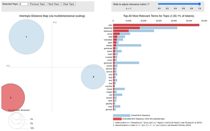
A side note here: the LDAvis R package can be used from R or RStudio but not directly from a notebook environment like Jupyter or Databricks. Therefore, we used the pyLDAvis port to the LDAvis package, since this makes it easy to include the wonderful LDAvis tool in a notebook. However, in some browsers the pyLDAvis is not working properly. If this happens, please see an example below. Feel free to download this notebook and try the LDAvis for yourself.
To run LDAvis locally with R or RStudio, you can run serVis(json) . To explore the interactive LDAvis from the screenprint below, see this link.

The left hand side plot shows the size of Topics (How many documents are attributed to the topic?) as well as the distance between Topics (What Topics are more/less related to each other?). The right hand side shows the important tokens for the selected Topic (or the overall most important tokens in the topic model when no topic is selected). With the top-right slider we can change lambda, where lambda decides how much we favor looking at the absolute token probability within the topic (p(token|topic), lambda = 1) or prefer the relative token probability within the topic (p(token|topic)/p(token), lambda = 0). Playing around with this visualization is often the best way to get familiar with the identified topics. And – most importantly – figuring out a proper topic label for each of the topics! This also is of great help in deciding whether the current topic model suffices for your downstream task or that you want to alter some settings (k, method, seed, …) or even the data (change selected documents or tokens) to get a better result.
Iterations towards your winning Topic Model
We said it before: topic modeling is – just like cluster analysis and other unsupervised machine learning techniques – more art than science! Therefore, you are probably going to spend quite some time tweaking your topic model before you end up with your ‘best’ Topic Model. We put ‘best’ in quotes here because what is ‘best’ depends heavily on both the applications you have in mind with your topic model and your creativity! So this is quite subjective! During the process of finding your ‘best’ topic model, you probably have some moments that you think you won’t come up with any solution you can use and other moments that you experience the ecstasy of seeing those intrinsic topics coming to live through the tokens that dominate it. In carving your optimal topic model, here are your most important tools:
- change k — the number of topics
- exclude extra ‘too dominant (frequent)’ tokens (these might still be too dominant and suppress finding more interesting subdomains in your text)
- increase the minimal token frequency to focus on the more dominant tokens
- sample documents to focus on the most relevant documents to find important topics, we could change the sampling strategy
Aside from these parameters, you also have some LDA parameters you can vary, but in our experience the parameters above are the most important ones to start with. Whereas increasing or decreasing k only means you have to re-estimate your LDA, changing the sampling of reviews or the tokens to consider means you also have to recreate your DTM.
What did we do? After lots of sweat, some cursing and exploring many solutions, we did the following:
- change k to 7 topics.
- Merge some tokens and exclude a number of too frequent tokens
- Explore multiple seed results (with nstart and best=FALSE) to find best interpretable topic model**
- Finally, select best seed and set best=TRUE to keep the best LDA model only
** The LDA function enables to do multiple runs by specifying the nstart parameter to set the number of runs and with seed set the seeds to guide these runs. When setting best=TRUE only the solution with the best log likelihood is preserved, setting it to best=FALSE enables you to explore all the topic models (the returned object is now a list of all topic models).
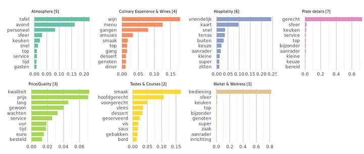
Iterating and comparing outcomes resulted in 7 topics we could label nicely with topic names of subjects that reviewers talk about when reviewing restaurants. Here’s our solution for the topics with the labels already added to them:
# modify the tokens to consider in topic model
reviews_tokens_train_smpl_new <- reviews_tokens_train %>%
  # remove infrequent tokens (<5)
  group_by(token) %>% mutate(token_freq=n()) %>%  filter(token_freq>=5) %>% ungroup() %>%
  # combine some tokens that are dominant in solutions and represent same meaning
  mutate(token = case_when(token == 'gerechten' ~ 'gerecht', token == 'wijnen' ~ 'wijn',
                           token == 'smaken' ~ 'smaak', token == 'vriendelijke' ~ 'vriendelijk',
                           TRUE~token)) %>%
  # remove some 'too frequent' tokens
  filter(!token  %in% c('goed','eten','restaurant','lekker','gegeten','komen','gaan','kregen',
                        'heerlijk','heerlijke','prima','kwam', 'mooi','mooie','leuk','leuke',
                        'lekker','lekkere','jammer','weinig','gezellig','gezellige','voldoende',
                        'uitstekend','attent','grote'))


# recreate the document term matrix after modifying the tokens to consider
dtm_new <- reviews_tokens_train_smpl_new %>%
    cast_dtm(document = restoReviewId,term = token,value = token_freq)

#check dimensions of dtm
cat(paste0('DTM dimensions: Documents (',dim(dtm_new)[1],') x Tokens (',dim(dtm_new)[2],')',
           ' (average token frequency: ',round(sum(dtm_new)/sum(dtm_new!=0),2),')'))

# estimate lda with k topics, set control variables nstart=n to have n runs,
#   best=FALSE to keep all run results and set the seed for reproduction
lda_fit_def <- LDA(dtm_new, k = 7,control = list(nstart=1,best=TRUE,seed=5678))
saveRDS(lda_fit_def,'lda_fit_def.RDS')
DTM dimensions:
Documents (10152) x Tokens (12496) (average token frequency: 416.26)
#since LDAvis package cannot be used in notebook, we use pyLDAvis, this can be used in notebook
# We need to export the R topic model output to use in python's pyLDAvis

# phi (topic - token distribution matrix) -  tokens in rows, topic scores in columns:
phi <- posterior(lda_fit_def)$terms %>% as.matrix

# theta (document - topic distribution matrix) -  documents in rows, topic probs in columns:
theta <- posterior(lda_fit_def)$topics %>% as.matrix

# number of tokens per document
doc_length <- reviews_tokens_train_smpl_new %>% group_by(restoReviewId) %>%
  summarize(doc_length=n()) %>% select(doc_length) %>% pull()

# vocabulary: unique tokens
vocab <- colnames(phi)

# overall token frequency
term_frequency <- reviews_tokens_train_smpl_new %>% group_by(token) %>%
  summarise(n=n()) %>% arrange(match(token, vocab)) %>% select(n) %>% pull()

# use tsne method to calculate distance between topics (default sometimes fails
# for details: https://www.rdocumentation.org/packages/LDAvis/versions/0.3.2/topics/createJSON)
library(tsne)
svd_tsne <- function(x) tsne(svd(x)$u)

# create JSON containing all needed elements
json <- createJSON(phi, theta, doc_length, vocab, term_frequency,mds.method=svd_tsne)

# render LDAvis - in RStudio, it opens a new window with the interactive LDAvis tool
serVis(json) # press ESC or Ctrl-C to kill
To explore the interactive LDAvis from the screenprint below, go to this html file.
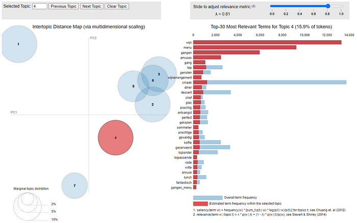
Although some topics are still a mix of things, we are happy to use this solution in predicting Michelin stars. We do see some clear distinctions between the identified topics and we expect that translating the raw text of each review into a vector of probabilities for these topics will help in predicting Michelin stars. Here’s an overview of the topics with the labels we give them and their most frequent tokens:
# get token probability per token per topic
topics <- tidy(lda_fit_def)

topiclabels <- data.frame(topic=seq(1,7),
                          label=c('Hospitality [6]','Tastes & Courses [2]',
                                  'Culinary Experience & Wines [4]','Atmosphere [5]',
                                  'Price/Quality [3]','Plate details [7]',
                                  'Waiter & Waitress [1]'))

# only select top-10 terms per topic based on token probability within a topic
plotinput <- topics %>%
  inner_join(topiclabels,by="topic") %>%
  group_by(label) %>%
  top_n(10, beta) %>%
  ungroup() %>%
  arrange(label, -beta)

# plot highest probability terms per topic
names <- levels(unique(plotinput$label))
colors <- RColorBrewer::brewer.pal(n=length(names),name="Set2")

plist <- list()

for (i in 1:length(names)) {
  d <- subset(plotinput,label == names[i])[1:10,]
  d$term <- factor(d$term, levels=d[order(d$beta),]$term)

  p1 <- ggplot(d, aes(x = term, y = beta, width=0.75)) +
  labs(title=names[i],y = NULL, x = NULL, fill = NULL) +
  geom_bar(stat = "identity",fill=colors[i]) +
  coord_flip() +
  guides(fill=FALSE) +
  theme_bw() + theme(strip.background  = element_blank(),
                     panel.grid.major = element_line(colour = "grey80"),
                     panel.border = element_blank(),
                     axis.ticks = element_line(size = 0),
                     panel.grid.minor.y = element_blank(),
                     panel.grid.major.y = element_blank(),
                     plot.title = element_text(size=7)) +
  theme(legend.position="bottom")

  plist[[names[i]]] = p1
}

library(gridExtra)
do.call("grid.arrange", c(plist, ncol=4))
Topic Modeling — wrapping it up
In this article we showed you how you can build a Topic Model to identify the latent constructs or ‘topics’ reviewers talk about in their restaurant reviews. As you have seen, there are quite some choices to be made before we have our final ‘best’ topic model and some of those choices are not easy to make since guiding statistics are not always available. Remember what we stated before: Topic modeling is an unsupervised technique and this makes it ‘more art that science’. What is important for many use cases is that you end up with topics you are able to interpret and explain, since you need to be able to interpret the features you’ve built here while using them in downstream tasks. With our 7-topic model, we feel confident we can do so!
Benefits
A great thing about topic modeling — and especially LDA — is that when all the tweaking and struggling is done, you are likely to end up with a manageable number of nicely interpretable topics. This allows you to add for each document the distribution over those topics. Since the topic probabilities sum to 1 and are numeric values, you now have summarized the unstructured, different length texts into just a few new, easy to process features. Features that can be of great value in downstream tasks like predictive modeling or segmentation tasks.
Drawbacks
The biggest drawback of topic modeling is most likely the subjectivity in finding the ‘best’ model. Therefore, it might take you quite some time and effort to come up with a proper topic model solution. There might be multiple statistically equivalent solutions that can differ substantially in the resulting topics. Therefore, when you rerun the analysis with slightly different data or settings, there is always the chance that the interpretation of the model is changed dramatically. Especially when no dominant topic solution is present in your textual data, each run might result in different results. Make sure you keep track of earlier runs, by securing seeds and datasets used so you won’t experience the frustration of finding a beautiful topic model solution you can nicely interpret en describe and then losing it to never restore it again.
Looking forward
Earlier, we’ve specified our goal: To predict what restaurants have a Michelin star. In one of our next blogs, we therefore use the distribution over topics in the review texts to predict whether the review is a Michelin review or not. We also aggregate those predictions over all reviews a restaurant has had to evaluate to what extent we are able to predict Michelin stars. Aside from this, we will use other techniques (word2vec, GloVe, BERT) to summarize the review texts into features we can use to predict Michelin stars and we’ll show what approach works best. We will start by introducing word embedding techniques (word2vec, GloVe) in our next blog and show you how to transform our review texts into embeddings and how to interpret and visualize those.
This article is of part of our NLP with R series. An overview of all articles within the series can be found here.
- Previous in this series: Data Preparation for Natural Language Processing
- Next up in this series: Training Word Embedding Model and Visualize Results
Do you want to do this yourself? Please feel free to download the Databricks Notebook or the R-script from out gitlab page.


